Weighted Agglomerative Clustering to Solve Normalized
Cuts Problems
Giulio Genovese
Mathematics Department, Dartmouth College, 6188 Kemeny Hall, Hanover, NH 03755, U.S.A.
Abstract. A new agglomerative algorithm is introduced that can be used as a re-
placement for any partitioning algorithm that tries to optimize an objective func-
tion related to graph cuts. In particular, spectral clustering algorithms fall in this
category. A new measure of similarity is introduced to show that the approach,
although radically different from the one adopted in partitioning approaches, tries
to optimize the same objective. Experiments are performed for the problem of im-
age segmentation but the idea can be applied to a broader range of applications.
1 Introduction
Many algorithms have been introduced in recent years that handle the problem of parti-
tioning a givenset of elements in a specified number k of groups. Among these, spectral
clustering [6–8], weighted kernel k-means [1–3] and non-negative matrix factorization
[4,9] have been proved to try to optimize the same objective function. Such an objective
function is related to a special kind of graph cuts, such as ratio cut and normalized cut,
that go under the broader name of weighted graph cuts. In this paper, we introduce a
new measure of similarity between subsets that gives a mathematical basis to prove that
it is possible to devise an agglomerative algorithm that tries to optimize the same math-
ematical function, adding another mathematically equivalent algorithm whose nature
and performance are although substantially different.
This novel algorithm is closely related to linkage clustering algorithms and, in the
case in which the objective function is related to ratio cuts, it is equivalent to average
linkage [5, Section 10.9.2]. We performed some experiments with objective functions
related to normalized cuts, in which case the algorithm resembles a sort of weighted
average linkage. Spectral algorithms have been applied to optimize normalized cuts for
the purpose of image segmentation. We tried to apply our new algorithm for the same
purpose obtaining some preliminary positive results that lead us to conclude that the
algorithm is competitive and deserving further study.
2 Normalized and Weighted Cuts
When clustering a dataset V = {x
1
, . . . , x
n
} through graph cuts, we think of the ele-
ments of our dataset as the vertices of a graph and we associate to each edge the value
corresponding to the affinity in between the two vertices. Suppose an affinity matrix A
is given, where A
ij
is the measure of affinity between element x
i
and element x
j
. We
Genovese G. (2008).
Weighted Agglomerative Clustering to Solve Normalized Cuts Problems.
In Proceedings of the 8th International Workshop on Pattern Recognition in Information Systems, pages 67-76
Copyright
c
 SciTePress

think of a partition {V
1
, . . . , V
k
} as a cut through the edges in between the subsets of
the partition. A cut will be optimal, then, according to the objective function we asso-
ciate to the cut. A bunch of objective functions are popular in the literature. We first
introduce the link between two subsets, not necessarily disjoint, as
l(A, B) =
X
x
i
∈A,x
j
∈B
A
ij
. (1)
Then we define the ratio association as an average measure of the clusters coherence
and ratio cut as an average measure of cluster affinity.
RAssoc(V
1
, . . . , V
k
) =
k
X
c=1
l(V
c
, V
c
)
|V
c
|
, RCut(V
1
, . . . , V
k
) =
k
X
c=1
l(V
c
, V \ V
c
)
|V
c
|
.
Despite the two functions being closely related, an optimal cut for ratio association is
not necessarily an optimal cut for ratio cut. To deal with this anomaly, the normalized
cut [8] has been introduced as
NCut(V
1
, . . . , V
k
) =
k
X
c=1
l(V
c
, V \ V
c
)
l(V
c
, V)
.
It is possible to define in an analogous way a normalized association but this is un-
necessary since it follows easily that the sum between normalized cut and normalized
association is constant. A generalization of these cuts is given by weighted cuts [3]. If
we introduce a weight function ω over the subsets of V, that is, a function such that for
every two disjoints subset A and B of V it holds
ω(A ∪ B) = ω(A) + ω(B), (2)
then the weighted association and the weighted cut are defined as
W Assoc(V
1
, . . . , V
k
) =
k
X
c=1
l(V
c
, V
c
)
ω(V
c
)
, W Cut(V
1
, . . . , V
k
) =
k
X
c=1
l(V
c
, V \ V
c
)
ω(V
c
)
.
It turns out that ratio association is a special case of weighted association for which the
weight function is just the set counting function, that is, ω(A) = |A| and the same can
be said for ratio cut. Also, the normalized cut is a special case of a weighted cut where
the weight function corresponds to the graph degree function, that is, ω(A) = l(A, V).
Other possible weights can be used but the ones just introduced have been the most
popular in the literature.
If the entries of the matrix A where ordered according to the clusters, Fig. 1 would
represent graphically the elements of the matrix A that are involved respectively with
the weighted cut and the weighted association.
Even if minimizing the weighted cut and maximizing the weighted association are
not in general equivalent problem, a strategy to maximize the weighted association is in
general sufficient. In fact, consider D the diagonal matrix whose diagonal elements are

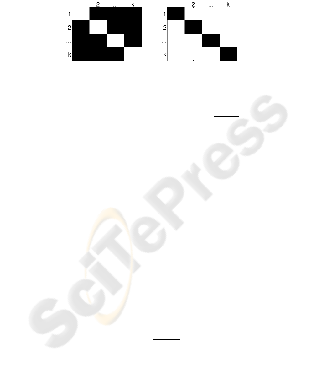
Fig.1. Weighted cut and weighted association.
the sum of the rows of matrix A. Then define the matrix A
′
= D − A as a new affinity
matrix and define
l
′
(A, B) =
X
x
i
∈A,x
j
∈B
A
′
ij
, W Assoc
′
(V
1
, . . . , V
k
) =
k
X
c=1
l
′
(V
c
, V
c
)
ω(V
c
)
.
It then follows easily that
W Assoc
′
(V
1
, . . . , V
k
) = W Cut(V
1
, . . . , V
k
),
and therefore a weighted cut can be interpreted as a weighted association for a different
affinity matrix. Notice that, even if the matrix A
′
is guaranteed to be semi-positive
definite, its components are mostly negative if the components of A are positive.
Spectral clustering (see [6] for a complete survey) can be seen as an algorithm to
maximize weighted association or to minimize weighted cuts. The algorithm is based on
an eigenvector decomposition of a matrix strictly related to the affinity matrix A. From
this decomposition the elements to be clustered are projected on a lower dimensional
vector space where a k-means algorithm separates them. Although, there is no qual-
ity guarantee for how well the objective function is optimized. Other approaches, like
weighted kernel k-means and non-negative matrix factorization [4], can at least guar-
antee that the solutions produced satisfy some local optimality conditions. For most
weighted cuts the problem of finding the optimal global solution is known to be NP -
hard. We are going to introduce an alternative method that optimizes the weighted cut
in a completely different way, but first we need to introduce a new way to measure the
similarity between two subsets.
3 Similarity Measures
Suppose we are given a set V with n elements and an n × n symmetric matrix A whose
component A
ij
represents the affinity between element x
i
and element x
j
. Suppose
also that we are given a weight function ω defined on the subsets of V and satisfying
(2) and the function l defined as in (1). Then a convenient way to measure the similarity
between two subsets A and B of V is to define a function S as
S(A, B) =
l(A, B)
ω(A)ω(B)
. (3)

This measure turns out to be strictly connected with weighted cuts. To begin with, notice
that, in case A and B are complementary and disjoint, that is, B = V \A, their similarity
is a constant multiple of the weighted cut, since
W Cut(A, B)
ω(A ∪ B)
= S(A, B).
In general it is true more.
Theorem 1. Given a partition {V
1
, . . . , V
k
} of a set V, the expressions
W Cut(V
1
, . . . , V
k
)
(k − 1)ω(V)
and
W Assoc(V
1
, . . . , V
k
)
ω(V)
are convex linear combinations of the pairwise similarities S(V
c
, V
d
) for c 6= d and the
self similarities S(V
c
, V
c
), respectively.
Proof. For the first expression, we have that
W Cut(V
1
, . . . , V
k
) =
k
X
c=1
l(V
c
, V \ V
c
)
ω(V
c
)
=
=
k
X
c=1
X
d6=c
ω(V
d
)
l(V
c
, V
d
)
ω(V
c
)ω(V
d
)
=
X
c<d
(ω(V
c
) + ω(V
d
))S(V
c
, V
d
)
and since it holds that
X
c<d
(ω(V
c
) + ω(V
d
)) = (k − 1)
k
X
c=1
ω(V
c
) = (k − 1)ω(V),
the convexity follows. For the second expression it is enough to show that
W Assoc(V
1
, . . . , V
k
) =
k
X
c=1
l(V
c
, V
c
)
ω(V
c
)
=
k
X
c=1
ω(V
c
)S(V
c
, V
c
).
Thanks to the previous theorem, if we have a strategy to minimize the pairwise simi-
larities between the k disjoint subsets that will finally form the partition we are looking
for, then we also have a strategy to minimize the weighted cut. The following theorem
leads to the algorithm we need.
Theorem 2. If the similarity measure S is defined as in (3), then it follows that

S(A, B) > S(A, C)
S(A, B) > S(B, C)
⇒ S(A, B) > S(A ∪ B, C). (4)
Proof. In fact, consider
S(A ∪ B, C) =
l(A ∪ B, C)
ω(A ∪ B)ω(C)
=
l(A, C) + l(B, C)
ω(A ∪ B)ω(C)
=
ω(A)
ω(A ∪ B)
l(A, C)
ω(A)ω(C)
+
ω(B)
ω(A ∪ B)
l(B, C)
ω(B)ω(C)
=
ω(A)S(A, C)
ω(A) + ω(B)
+
ω(B)S(B, C)
ω(A) + ω(B)
,

so that S(A ∪ B, C) is a convex linear combination of values that are both smaller than
S(A, B), making it smaller as well.
The property (4) is very important since it means that every time we join the two most
similar clusters, the pairwise similarities in between the new cluster get smaller. This
provides a basis for an agglomerative clustering algorithm. The idea is simple. At the
beginning every element forms a different cluster and at every step we join the two
clusters for which the similarity measure is the largest until we are left with k clusters.
This way we make sure that the largest pairwise cluster similarity gets smaller at every
step. Even if this does not guarantee an optimal solution for the weighted cut in the
end, which in general is NP -hard to find, it does justify agglomerative clustering as a
possible strategy.
Algorithm 1: Weighted agglomerative algorithm.
Input: Set V = {x
1
, . . . , x
n
}, affinity matrix A, and list of weights.
Initialize
ˆ
k ← n and clusters V
i
← {x
i
}.
repeat
ˆ
k ←
ˆ
k − 1
Find clusters V
c
and V
d
for which S(V
c
, V
d
) is minimal.
Join cluster V
c
and cluster V
d
.
Compute similarities between the new cluster and the other clusters.
until k =
ˆ
k
Agglomerative clustering is a common tool for data clustering. It can be proved
that average linkage [5, Section 10.9.2] is equivalent to the agglomerative algorithm
previously described where we choose as weight the element counting weight, that is,
ω(V
c
) = |V
c
|. Usually agglomerative clustering deals with distances, or dissimilarities,
instead of similarities, but the idea is basically the same.
4 Iterative Optimization
If our goal is to find the partition {V
1
, . . . , V
k
} that maximizes the weighted association,
then this is equivalent to minimizing the quantity
W Assoc({x
1
}, . . . , {x
n
}) − W Assoc(V
1
, . . . , V
k
), (5)
since the first term is just a constant independent of the partition. Define the divergence
between two clusters A and B as
D(A, B) = S(A, A) − 2S(A, B) + S(B, B).
Theorem 3. The quantity in (5) is equal to the sum
k
X
c=1
X
x
i
∈V
c
ω(x
i
)D({x
i
}, V
c
). (6)
71

Proof. Rewrite the quantity in (5) as
W Assoc({x
1
}, . . . , {x
n
}) −
k
X
c=1
ω(V
c
)S(V
c
, V
c
) =
= W Assoc({x
1
}, . . . , {x
n
}) − 2
k
X
c=1
ω(V
c
)S(V
c
, V
c
) +
k
X
c=1
ω(V
c
)S(V
c
, V
c
) =
= W Assoc({x
1
}, . . . , {x
n
}) − 2
k
X
c=1
X
x
i
∈V
c
ω(x
i
)S({x
i
}, V
c
) +
k
X
c=1
ω(V
c
)S(V
c
, V
c
) =
=
X
x
i
∈V
ω(x
i
)S({x
i
}, {x
i
}) − 2
k
X
c=1
X
x
i
∈V
c
ω(x
i
)S({x
i
}, V
c
) +
k
X
c=1
ω(V
c
)S(V
c
, V
c
) =
=
k
X
c=1
X
x
i
∈V
c
ω(x
i
)(S({x
i
}, {x
i
}) − 2S({x
i
}, V
c
) + S(V
c
, V
c
))
and the last expression is the same as (6).
The previous expression, by trying to measure separately the contribution of each el-
ement, suggests an iterative strategy to optimize the weighted association. If we think
of our elements as points in a Euclidean space, and if the weights are all equal to 1
and the divergence D coincides with the squared distance between the centroids, then
the expression coincides with the sum of squared error [5, Section 10.7.1], that is, the
objective function that is being minimized by the k-means algorithm.
We can therefore use ideas from the k-means literature to improve a givenclustering
obtained with the agglomerative approach used in the previous section. In particular, it
is possible to generalize a common iterative optimization for k-means [5, Section 10.8]
to optimize the weighted association. To this purpose, we first need a lemma.
Lemma 1. If A is a cluster and x is an element of V that does not belong to the cluster
A, then the following holds
W Assoc(A, {x}) − W Assoc(A ∪ {x}) =
ω(A)
ω(A ∪ {x})
ω({x})D({x}, A) =
ω(A ∪ {x})
ω(A)
ω({x})D({x}, A ∪ {x}).
A proof can be found in the appendix. The previous lemma provides an easy rule
for improving the weighted association. In fact, suppose we have an element x assigned
to cluster A and suppose we are wondering if it would be better to assign it to cluster
B. We just need to check if
W Assoc(A, B) < W Assoc(A \ {x}, B ∪ {x}).
By the lemma, this is equivalent to check if
ω(A)
ω(A \ {x})
D({x}, A) <
ω(B)
ω(B ∪ {x})
D({x}, B).

Therefore, if we keep updated the element-to-cluster similarities, it is easy to compute
the element-to-cluster divergences and to check if the above equation holds. This leads
to a natural iterative algorithm.
Algorithm 2: Weighted iterative algorithm.
Input: Set V = {x
1
, . . . , x
n
}, partition {V
1
, . . . , V
k
}, list of weights, and element-to-cluster
similarities S({x
i
}, V
c
).
for all x
i
∈ V do
if x
i
∈ V
c
and there is a cluster V
d
for which
ω(V
c
)D({x
i
},V
c
)
ω(V
c
\{x
i
})
<
ω(V
d
)D({x
i
},V
d
)
ω(V
d
∪{x
i
})
, then
Reassign x
i
from cluster V
c
to cluster V
d
.
Update the element-to-cluster similarities and the element-to-cluster divergences.
end if
end for
Such an algorithm can be run at any time during the running of the previous algo-
rithm. The algorithm is guaranteed to stop since at every step the weighted association
of the partition increases. Although, many steps might be required before converging to
a local optimum. One way to deal with this is to use weighted kernel k-means, which
performs many reassignments at once, but if the similarity matrix S({x
i
}, {x
j
}) is not
positive definite, then you are not guaranteed to improve the weighted association and
some tricks might be required to enforce positive definiteness [3]. A related algorithm
has been implemented inside the kmeans function in the MATLAB statistical toolbox
where it is left to the user to decide if running it or not once the k-means algorithm has
converged. In fact, depending on the number of elements and clusters, it might be more
or less appropriate to perform this iterative procedure since it can be time consuming.
5 Experimental Results
Experimental results on images have given positive results. Moreover, the weighted
approach using normalized cuts, compared to the unweighted approach using ratio cuts,
has showed to be less likely to generate clusters of small sizes.
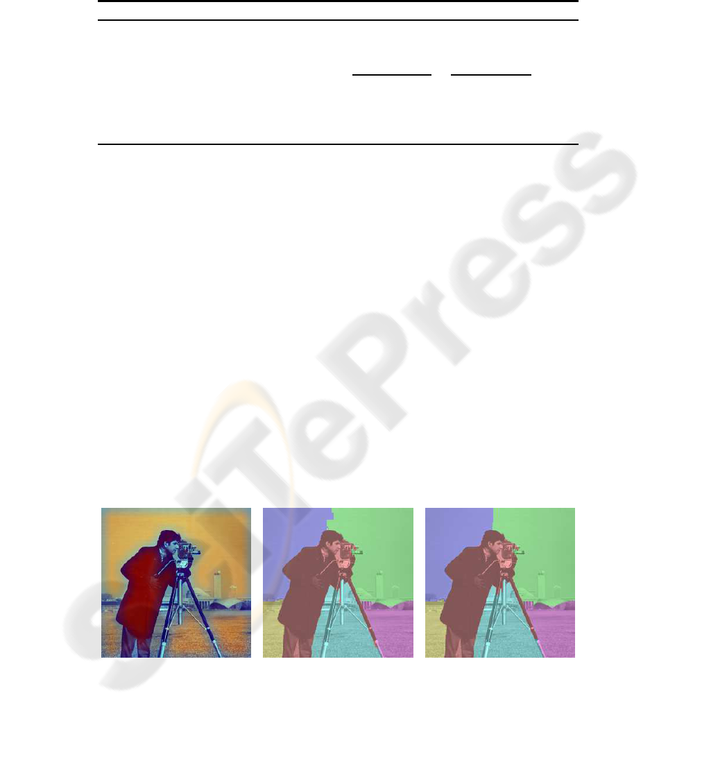
Fig.2. First test image.
73

To show the results of our algorithm, we picked the left picture in Fig. 2 as a test
figure. We used as the affinity matrix the one built with Yu’s software [10]. In the image
we intensified with red the pixels with large weight, as a result of the particular affinity
matrix chosen, and with blue the pixels with small weight. We then run the agglomer-
ative algorithm with k = 6, the target amount of clusters. The resulting segmentation
is shown in the central picture. The value of the normalized cut turned out to be 0.055.
Using the iterative optimization algorithm starting from the previous partitioning, we
obtained the refined clustering shown in the right picture. The value of the normalized
cut dropped, as expected, to 0.046.
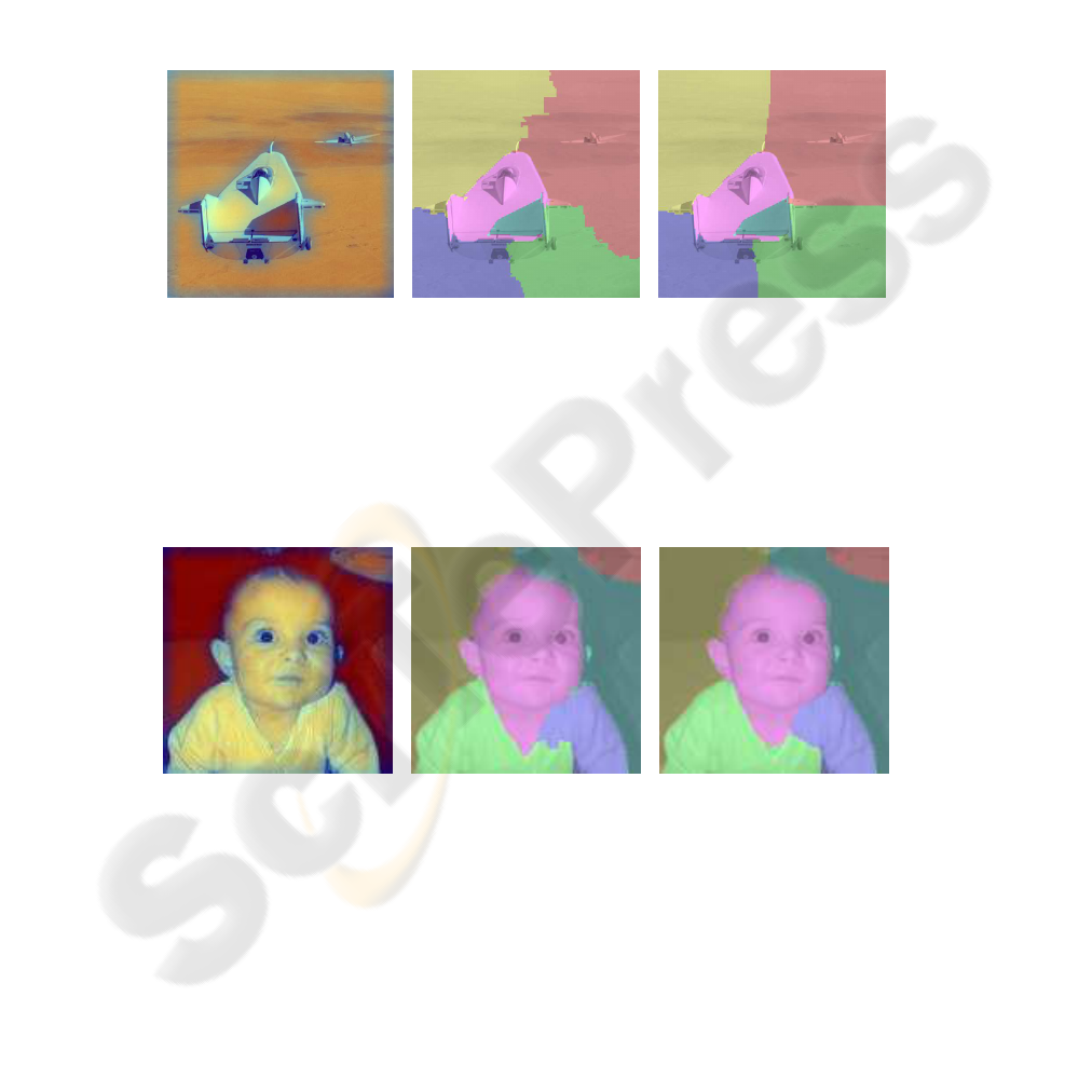
Fig.3. Second test image.
A second example, using the left picture in Fig. 3, was used to show how the re-
fining process can change dramatically the original partition. The initial segmentation
is shown in the central picture. The value of the normalized cut was in this case 0.219.
Using the iterative optimization algorithm produced the partition shown in the right
picture. In this case the value of the normalized cut dropped to 0.172.
Fig.4. Third test image.
To show another example, we picked the left picture in Fig. 4 and we run again
the agglomerative algorithm. The resulting partitioning is shown in the central picture
with value 0.189 for the normalized cut. The iterative optimization improved the value
of the normalized cut to 0.170, producing the right picture. In all cases the iterative
optimization provided a clear visual improvement of the cuts, although it should be

noticed that the amount of pixels that could end up being moved can be very large
suggesting that it is important to initiate the algorithm from a partitioning that is already
good.
Even if the similarity matrix was sparse, we didn’t take advantage of this fact due
to lack of time to code a sparse approach for the weighted agglomerative algorithm,
so we preferred to omit running times. Although, experiments have shown that the al-
gorithm is fast and practical and a sparse version would definitely make it competitive
with a sparse spectral approach. All of the code used in the experiment has been writ-
ten in MATLAB and C++ and is freely available on the author’s website at the URL
http://www.math.dartmouth.edu/∼genovese/.
6 Conclusions
A new agglomerative algorithm for clustering data has been proposed. Despite the fact
that the algorithm has been proved to try to optimize the same objective function as
k-means like algorithms, it is meant more as a complement rather than a substitute to
partitioning algorithms. Many practical algorithms that deal with large datasets apply
partitioning algorithms after coarsening the data enough to make the approach feasi-
ble. The mathematical framework here introduced justifies the weighted agglomerative
approach as an algorithm to perform the coarsening.
An important direction of investigation would be the one of changing the weights
associated to the elements. We have chosen the weights that best optimize the normal-
ized cut objective function but any kind of weight would have delivered a different and
possible algorithm and understanding better this choice might help deciding which al-
gorithm should fit best the problem that is being tackled. In the clustering literature
usually it is the case that some elements act as exemplars for other elements and maybe
an appropriate weighting is exactly the right way to measure this fact.
Acknowledgements
This work is supported by NIH, grant number NIH R01GM075310-02.
References
1. I. Dhillon, Y. Guan, and B. Kulis, (2004), Kernel k-means: spectral clustering and normal-
ized cuts, In KDD ’04: Proceedings of the tenth ACM SIGKDD international conference on
Knowledge discovery and data mining, pages 551–556, New York, NY, USA. ACM.
2. I. Dhillon, Y. Guan, and B. Kulis, (2005). A fast kernel-based multilevel algorithm for graph
clustering. In KDD ’05: Proceeding of the eleventh ACM SIGKDD international conference
on Knowledge discovery in data mining, pages 629–634, New York, NY, USA. ACM.
3. I. Dhillon, Y. Guan, and B. Kulis, (2007). Weighted Graph Cuts without Eigenvectors A
Multilevel Approach, IEEE Trans. Pattern Anal. Mach. Intell., 29(11):1944–1957.
4. C. Ding, X. He, and H. D. Simon, (2005). On the equivalence of nonnegative matrix factor-
ization and spectral clustering. In Proc. SIAM Data Mining Conf., pages 606–610.

5. R. O. Duda and P. E. Hart, and D. G. Stork, (2000), Pattern Classification, 2nd ed., John
Wiley and Sons.
6. Ulrike Luxburg, (2007), A tutorial on spectral clustering, Statistics and Computing,
17(4):395–416.
7. A. Ng, M. Jordan, and Y. Weiss, (2001). On spectral clustering: Analysis and an algorithm.
In Advances in Neural Information Processing Systems 14: Proceedings of the 2001.
8. J. Shi and J. Malik, (2000), Normalized cuts and image segmentation, Transactions on Pattern
Analysis and Machine Intelligence, 22(8):888-905.
9. W. Xu, X. Liu, and Y. Gong, (2003). Document clustering based on non-negative matrix
factorization. In SIGIR ’03: Proceedings of the 26th annual international ACM SIGIR con-
ference on Research and development in information retrieval, pages 267–273, New York,
NY, USA. ACM.
10. Stella Yu, (2003). Computational Models of Perceptual Organization. PhD thesis, Robotics
Institute, Carnegie Mellon University, Pittsburgh, PA. CNBC and HumanID.
Appendix
A proof of lemma 1 is given.
W Assoc(A, {x}) − W Assoc(A ∪ {x}) =
= ω(A)S(A, A) + ω({x})S({x}, {x}) − ω(A ∪ {x})S(A ∪ {x}, A ∪ {x}).
For the first equality rewrite the last expression as
ω(A)S(A, A) + ω({x})S({x}, {x}) − ω(A)S(A, A ∪ {x})
− ω({x})S({x}, A ∪ {x}) =
= ω(A)S(A, A) + ω({x})S({x}, {x}) −
ω(A)
2
S(A, A) + ω(A)ω({x})S(A), {x}
ω(A ∪ {x})
−
ω(A)ω({x})S({x}, A) + ω({x})
2
S({x}, {x})
ω(A ∪ {x})
=
=
ω(A)
ω(A ∪ {x})
ω({x})(S({x}, {x}) − 2S({x}, A) + S(A, A)) =
=
ω(A)
ω(A ∪ {x})
ω({x})D({x}, A).
For the second equality rewrite the previous expression as
ω(A ∪ {x})S(A ∪ {x}, A) − ω({x})S({x}, A)
+ ω({x})S({x}, {x}) − ω(A ∪ {x})S(A ∪ {x}, A ∪ {x}) =
=
ω(A ∪ {x})
2
S(A ∪ {x}, A ∪ {x})
ω(A)
−
2ω(A ∪ {x})ω({x})S({x}, A ∪ {x})
ω(A)
+
ω({x})
2
S({x}, {x})
ω(A)
+ ω({x})S({x}, {x}) − ω(A ∪ {x})S(A ∪ {x}, A ∪ {x}) =
=
ω(A ∪ {x})
ω(A)
ω({x})(S({x}, {x}) − 2S({x}, A ∪ {x}) + S(A ∪ {x}, A ∪ {x})) =
=
ω(A ∪ {x})
ω(A)
ω({x})D({x}, A ∪ {x}).