
NEW APPROACHES TO CLUSTERING DATA
Using the Particle Swarm Optimization Algorithm
Ahmed Ali Abdalla Esmin
Department of Computer Science (DCC), Federal University of Lavras (UFLA), Brazil
Dilson Lucas Pereira
Department of Computer Science (DCC), Federal University of Lavras (UFLA), Brazil
Keywords: PSO, Data clustering.
Abstract: This paper presents a new proposal for data clustering based on the Particle Swarm Optimization Algorithm
(PSO). In the PSO algorithm, each individual in the population searches for a solution taking into account
the best individual in a certain neighbourhood and its own past best solution as well. In the present work, the
PSO algorithm was adapted by using different finenesses functions and considered the situation where the
data is uniformly distributed. It is shown how PSO can be used to find the centroids of a user specified
number of clusters. The proposed method was applied in an unsupervised fashion to a number of benchmark
classification problems and in order to evaluate its performance.
1 INTRODUCTION
The amount of available data and information
collected nowadays is greater than the human
capability to analysis and extracting knowledge from
it. To helpful in the analysis and to extract
knowledge efficiently and automatically new
techniques and new algorithms need to be
developed.
Clustering is an important problem that must often
be solved as a part of more complicated tasks in
pattern recognition, image analysis and other fields
of science and engineering. Clustering, is one of the
main tasks of knowledge discovery from databases
(KDD) (Fayyad, 1996), and consists of finding
groups within a certain set of data in which each
group contains objects similar to each other and
different from those of other groups (Fayyad 1996),
(Jiawei, 2001) and (Fränti, 2002).
In the most of real-world applications the data
bases are very large, with high dimensions, contain
attributes of different domains. The computational
cost of clustering is crucial, and brute force
deterministic algorithms are not appropriate in most
of these real-world cases.
Clustering algorithms can be divided into two
main classes of algorithms (supervised and
unsupervised). In supervised clustering, the learning
algorithm is provided with both the cases (data
points) and the labels that represent the concept to be
learned for each case (has an external teacher that
indicates the target class to which a data vector
should belong). On the other hand, in unsupervised
clustering, the learning algorithm is provided with
just the data points and no labels, the task is to find a
suitable representation of the underlying distribution
of the data (a teacher does not exist, and data vectors
are grouped based on distance from one another).
This paper focuses on unsupervised clustering.
Particle Swarm Optimization (PSO) algorithm is a
novel optimization method developed by Eberhart et
al (Kennedy and Eberhart, 1995). PSO finds the
optimal solution by simulating social behaviors of
groups as fish schooling or bird flocking. This
means that, PSO is an optimization method that uses
the principles of social behavior. A group can
effectively achieve its objective by using the
common information of every agent, and the
information owned by the agent itself. PSO has
proved to be competitive with Genetic Algorithms in
several tasks, mainly in optimization areas. (Esmin,
593
Ali Abdalla Esmin A. and Lucas Pereira D. (2008).
NEW APPROACHES TO CLUSTERING DATA - Using the Particle Swarm Optimization Algorithm.
In Proceedings of the Tenth International Conference on Enterprise Information Systems - AIDSS, pages 593-597
DOI: 10.5220/0001722105930597
Copyright
c
SciTePress

2005).
This paper presents a new proposal for data
clustering based on the Particle Swarm Optimization
Algorithm (PSO). The PSO algorithm was adapted
by using different finenesses functions and
considered the situation where the data is uniformly
distributed.
The remainder of the paper is organized as
follows: Section II presents an overview about the
PSO, Section III the PSO clustering algorithm is
presented and Section IV shows the tests and the
performance analysis. Finally, the conclusions are
presented.
2 AN OVERVIEW OF PSO
The Particle Swarm Optimization Algorithm (PSO)
is a population-based optimization method that finds
the optimal solution using a population of particles
(Kennedy and Eberhart, 1995). Every swarm of PSO
is a solution in the solution space. PSO is basically
developed through simulation of bird flocking in a
two-dimensional space. The PSO definition is
presented as follows:
Each individual particle i has the following
properties: A current position in search space, x
i
, a
current velocity, v
i
, and a personal best position in
search space, y
i
.
The personal best position, y
i
, corresponds to the
position in search space where particle i presents the
smallest error as determined by the objective
function f, assuming a minimization task.
The global best position denoted by
y
(
represents
the position yielding the lowest error amongst all the
y
i
.
Equations (1) and (2) define how the personal and
global best values are updated at time t, respectively.
It is assumed below that the swarm consists of s
particles, Thus
si ..1∈
.
⎩
⎨
⎧
+>+
+≤
=+
)))1(()(()1(
)))1(()(()(
)1(
txftyfiftx
txftyfifty
ty
iii
iii
i
(1)
{}
}{
)(),.....,(),(
))((),(min)(
10
tytytyy
tyfyfty
s
∈
=
((
(2)
During the iteration every particle in the swarm is
updated using equations (3) and (4). The velocity
update step is:
)]()()[(
)]()()[()()1(
,,22
,,,11,,
txtytrc
txtytrctwvtv
jijj
jijijjiji
−
+−
+
=
+
(
(3)
The current position of the particle is updated to
obtain its next position:
)1()()1( +
+
=
+
tvtxtx
iii
(4)
where, c
1
and c
2
are two positive constants, r
1
and
r
2
are two random numbers within the range [0,l],
and w is the inertia weight.
The equation (3) consists of three parts. The first
part is the former speed of the swarm, which shows
the present state of the swarm; the second part is the
cognition modal, which expresses the thought is the
cognition modal, which expresses the thought of the
swarm itself; the third part is the social modal. The
three parts together determine the space searching
ability. The first part has the ability to balance the
whole and search a local part. The second part
causes the swarm to have a strong ability to search
the whole and avoid local minimum. The third part
reflects the information sharing among the swarms.
Under the influence of the three parts, the swarm can
reach an effective and best position.
3 PSO CLUSTERING
There are some works from the literature that
modify the particle swarm optimization algorithm to
solve clustering problems.
In the work (Merwe 2003) and (Cohen 2006),
each particle corresponds to a vector containing the
centroids of the clusters. Initially, particles are
randomly created. For each input datum, the winning
particle (i.e., the one that is closer to the datum) is
adjusted following the standard PSO updating
equations. Thus, differently from the k-means
algorithm, several initializations are performed
simultaneously. The authors also investigated the
use of k-means to initialize the particles.
Experiments were performed with two artificially
generated data sets, and some benchmark
classification tasks were also investigated. The
method is based on a cost function that evaluates
each candidate solution (particle) based on the
proposed clusters’ centroids.
The particle X
i
is constructed as follows:
X
i
= (m
i1
, m
i2
, …, m
ij
, …, m
iNc
)
where Nc is the number of clusters to be formed and
m
ij
corresponds to the j
th
centroid of the i
th
particle,
the centroid of the cluster C
ij
. Thus, a single particle
represents a candidate solution to a given clustering
ICEIS 2008 - International Conference on Enterprise Information Systems
594

problem. Each particle is evaluated using the
following equation:
Nc
Cmzd
J
c
ijp
N
jCZ
ijijp
e
∑∑
=∈∀
=
1
]||/).([
(F1)
where Zp denotes the p
th
data vector, | C
ij
| is the
number of data vectors belonging to the cluster C
ij
and d is the Euclidian distance between Zp and m
ij
.
3.1 The Evaluation Function
The Evaluation function plays a fundamental role in
any evolutionary algorithm; it tells how good a
solution is.
By analyzing the equation F1 we can see that it is
first takes each cluster C
ij
and calculates the average
distance of the data belonging to the cluster to its
centroid m
ij
. Then it takes the average distances of
all clusters C
ij
and calculates another average, which
is the result of the equation.
It can be seen that a cluster C
ij
with just one data
vector will influence the final result (the quality) as
much as a cluster C
ik
with lot of data vectors.
Sometimes a particle that does not represent a
good solution is going to be evaluated as if it did.
For instance, suppose that one of the particle clusters
has a data vector that is very close to its centroid,
and another cluster has a lot of data vectors that are
not so close to the centroid. This is not a very good
solution, but giving the same weight to the cluster
with one data vector as the cluster with a lot of data
vectors can make it seem to be. Furthermore, this
equation is not going to reward the homogeneous
solutions, that is, solutions where the data vectors
are well distributed along the clusters.
To solve this problem we propose the following
new equations, where the number of data vectors
belonging to each cluster is taken into account:
∑∑
=∈∀
×=
c
ijp
N
j
oij
CZ
ijijp
NCCmzdF
1
)]}/|(|)||/).([({
(F2)
Where N
o
is the number of data vectors to be
clustered.
To take into account the distribution of the data
among the clusters, the equation can be changed to:
)1|||(|' +−×= ilik CCFF
(F3)
such that,
|}{|max|| ,..,1 ijNcjik CC =∀=
and
|}{|min|| ,..,1 ijNcjil CxC =∀=
The next section shows the test results with these
different equations.
4 RESULTS
Table 1 shows the three benchmarks that used: Iris,
Wine and Glass, taken from the UCI Repository of
Machine Learning Databases. (Assuncion, 2007).
Table 1: Benchmarks features.
Benchmark Number of
Objects
Number of
Attributes
Number
of
Classes
Iris 150 4 3
Wine 178 13 3
Glass 214 9 7
For each data set, three implementations, using the
equations F1, F2 and F3, were run 30 times, with
200 function evaluations and 10 particles, w = 0.72,
c1 = 1.49, c2 = 1.49. (Merwe 2003).
Each benchmark class is represented by the
particle created cluster with largest number of data
of that class; data of different classes within this
cluster are considered misclassified. Thus the hit rate
of the algorithm can be easily calculated.
The average hit rate t over the 30 simulations ±
the standard deviation σ of each implementation is
presented in Table 2.
As can be seen on Table 2 the changes on the
fitness function brought good improvements to the
results on the evaluated benchmarks. It is important
to notice that equation F3 pushes the particles
towards clusters with more uniformly distributed
data, so it should be used on problems in witch is
previously known that clusters have uniform
distribution sizes, otherwise, equation F2 should be
used. On Iris, in witch clusters have uniform sizes,
equation F3 produced very good results, even
though equation F2 produced good results too. The
improvements on the others benchmarks are also
satisfactory.
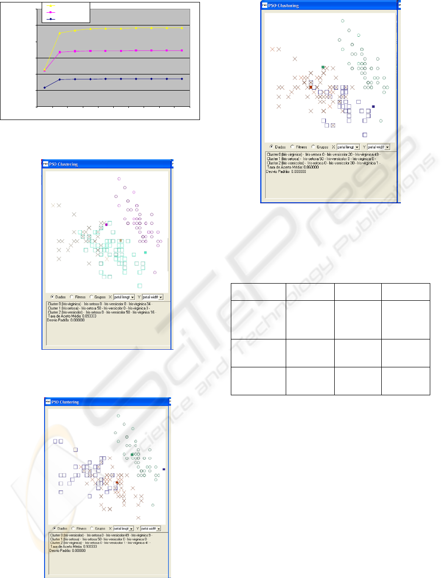
On Figure 1, the convergence of the three
functions is shown. As a characteristic of the PSO,
they all have a fast convergence.
On Figures 2, 3 and 4, some examples of
clustering found can be seen. On Figure 2 contains
some examples of clustering for the Iris benchmark,
on the algorithm using function F1 found the correct
group for 71,9% of data, on Figure 3 the F2 found
the correct group for 88,6%, and on Figure 4 the F3
found the correct group for 85,3%. It can be seen
that F2 and F3 totally distinguished the class setosa
(squares) from the other classes.
NEW APPROACHES TO CLUSTERING DATA - Using the Particle Swarm Optimization Algorithm
595
0,0000000000
0,0000001000
0,0000002000
0,0000003000
0,0000004000
0,0000005000
0,0000006000
0 22 44 66 88 111 133 155 177 199
Iteration
Fitnes
s
Fitness Function F3
Fitness Function F2
Fitness Function F1
Figure 1: fitness curve of the implementations along the
iterations.
Figure 2: Example of Clustering found by implementation
using equation F1 to Iris benchmark (Petal Length x Petal
Width).
Figure 3: Example of Clustering found by implementation
using equation F2 to Iris benchmark (Petal Length x Petal
Width).
Figure 4: Example of Clustering found by implementation
using equation F3 to Iris benchmark (Petal Length x Petal
Width).
Table 2: Comparison of the results using fitness function
F1, F2 and F3.
Benchmark F1 F2 F3
Iris 66.6444%
± 9.6156%
83.1333%
± 8.4837%
88.3778%
±
10.6421%
Wine 68.9139%
± 6.4636%
71.2172%
± 0.5254%
71.8726%
± 0.1425%
Glass 42.3053%
± 5.1697%
46.3396%
± 3.7626%
43,3178%
± 3,4833%
5 CONCLUSIONS
This work proposed different approaches to
clustering data by using the PSO algorithms.
Three well known benchmarks were used to
compare the efficiency of these three methods; the
average hit rate was used to compare them. The
results show that significant improvements were
achieved by the implementations using the proposed
modifications.
Among the many issues to be further investigated,
the automatic determination of an optimal number of
particles, handling complex shaped clusters and the
automatic partition of the clusters are three of the
most important issues.
ICEIS 2008 - International Conference on Enterprise Information Systems
596

ACKNOWLEDGEMENTS
To FAPEMIG and CNPq for supporting this work.
REFERENCES
Asuncion, A & Newman, D.J. (2007). UCI Machine
Learning Repository Irvine, CA: University of
California, Department of Information and Computer
Science.[http://www.ics.uci.edu/~mlearn/MLRepositor
y.html].
Cohen, S. C. M.; Castro, L. N. de. Data Clustering with
Particle Swarms. In: Congress on Evolutionary
Computation, 2006. Proceedings of IEEE Congress on
Evolutionary Computation 2006 (CEC 2006).
Vancouver: IEEE Computer Society, 2006. p. 1792-
1798.
Eberhart, R. C. and Kennedy, J. . A new optimizer using
particle swarm theory. In Proceedings of the Sixth
International Symposium on Micro Machine and
Human Science, Nagoya, Japan, pp. 39-43, 1995.
Esmin, A. A. A. ; Lambert-Torres, G. ; Souza, Antonio
Carlos Zambroni de . A Hybrid Particle Swarm
Optimization Applied to Loss Power Minimization.
IEEE Transactions on Power Systems, V. 20, n. 2, p.
859-866, 2005.
Fayyad, U.M., Piatetsky-Shapiro, G., Smyth, P.,
Uthurusamy, R. (1996), “Advances in Knowledge
Discovery and Data Mining”, Chapter 1, AAAI/MIT
Press 1996.
Fränti, O. Virmajoki and Kaukoranta T., "Branch-and-
bound technique for solving optimal clustering", Int.
Conf. on Pattern Recognition (ICPR'02), Québec,
Canada, vol. 2, 232-235, August 2002.
Kennedy, J. and Eberhart, R. C.. Particle Swarm
Optimization. In Proceedings of IEEE Internal
Conference on Neural Networks, Perth, Australia,Vol.
4, pp. 1942- 1948, 1995.
Jiawei, H., Micheline, K. (2001), “Data Mining, Conecpts
and Techniques”, Morgan Kaufmann Publishers.
Merwe, D. W. van der; Engelbrecht, A. P. Data Clustering
using Particle Swarm Optimization . In: Congress on
Evolutionary Computation, 2003. Proceedings of
IEEE Congress on Evolutionary Computation 2003
(CEC 2003), Caribella: IEEE Computer Society, 2003.
p. 215-220.
NEW APPROACHES TO CLUSTERING DATA - Using the Particle Swarm Optimization Algorithm
597
