SIZE AND EFFORT-BASED COMPUTATIONAL MODELS FOR

SOFTWARE COST PREDICTION

Efi Papatheocharous and Andreas S. Andreou

University of Cyprus, Dept. of Computer Science

75 Kallipoleos str., CY1678 Nicosia, Cyprus

Keywords: Artificial Neural Networks, Genetic Algorithms, Software Cost Estimation.

Abstract: Reliable and accurate software cost estimations have always been a challenge especially for people involved

in project resource management. The challenge is amplified due to the high level of complexity and

uniqueness of the software process. The majority of estimation methods proposed fail to produce successful

cost forecasting and neither resolve to explicit, measurable and concise set of factors affecting productivity.

Throughout the software cost estimation literature software size is usually proposed as one of the most

important attributes affecting effort and is used to build cost models. This paper aspires to provide size and

effort-based estimations for the required software effort of new projects based on data obtained from past

completed projects. The modelling approach utilises Artificial Neural Networks (ANN) with a random

sliding window input and output method using holdout samples and moreover, a Genetic Algorithm (GA)

undertakes to evolve the inputs and internal hidden architectures and to reduce the Mean Relative Error

(MRE). The obtained optimal ANN topologies and input and output methods for each dataset are presented,

discussed and compared with a classic MLR model.

1 INTRODUCTION

Accurate software development cost estimation has

always been a major concern especially for people

involved in project management, resource control

and schedule planning. A good and reliable estimate

could provide more efficient management over the

whole software process and guide a project to

success. The track record of IT projects shows that

often a large number fails. Most IT experts agree

that such failures occur more regularly than they

should (Charette, 2005). According to the 10

edition of the annual CHAOS report from the

Standish Group that studied over 40,000 projects in

10 years, success rates increased to 34% and failures

declined to 15% of the projects. However, 51% of

the projects overrun time, budget and/or lack critical

features and requirements, while the average cost

apparently overruns by 43% (Software Magazine,

2004). One of the main reasons for these figures is

failure to estimate the actual effort required to

develop a software project.

The problem is further amplified due to the high

level of complexity and uniqueness of the software

process. Estimating software costs, as well as

choosing and assessing the associated cost drivers,

both remain difficult issues that are constantly at the

forefront right from the initiation of a project and

until the system is delivered. Cost estimates even for

well-planned projects are hard to make and will

probably concern project managers long before the

problem is adequately solved.

Over the years software cost estimation has

attracted considerable research attention and many

techniques have been developed to effectively

predict software costs. Nonetheless no single

solution has yet been proposed to address the

problem. Typically, the amount and complexity of

the development effort proportionally drives

software costs. However, as other factors, such as

technology shifting, team and manager skills,

quality, size etc., affect the development process it is

even more difficult to assess the actual costs.

A commonly investigated approach is to

accurately estimate some of the fundamental

characteristics related to cost, such as effort, usually

measured in person-months. However, it is preferred

to measure a condensed set of attributes and then use

them to estimate the actual effort. Software size is

commonly recognised as one of the most important

factors affecting the amount of effort required to

complete a project according to Fenton and Pfleeger

Papatheocharous E. and S. Andreou A. (2008).

SIZE AND EFFORT-BASED COMPUTATIONAL MODELS FOR SOFTWARE COST PREDICTION.

In Proceedings of the Tenth International Conference on Enterprise Information Systems - DISI, pages 57-64

DOI: 10.5220/0001708800570064

 SciTePress

(1997). It is considered a fairly unpromising metric

to provide early estimates mainly because it is

unknown until the project terminates. Nonetheless,

many researchers investigate cost models using size

to estimate effort (e.g.,Wittig and Finnie; Dolado

2001) whereas others direct their efforts towards

defining concise methods and measures to estimate

software size from the early project phases (e.g.,

Park 2005; Albrecht 1979). The present work is

related to the former, aspiring to provide size and

effort-based estimations for the software effort

required for a new project using data from past

completed projects, even though they originate back

from the 90’s. The hypothesis is that once a robust

relationship between size and effort is affirmed by

means of a model, then this model may be used

along with size estimations to predict effort of new

projects more accurately. Thus, in this work we

attempt to study the potentials of developing a

software cost model using computational

intelligence techniques relying only on size and

effort data. The core of the model proposed consists

of Artificial Neural Networks (ANN). The ANN’s

architecture is further optimised with the use of a

Genetic Algorithm (GA), focused on evolving the

number and type of inputs, as well as the internal

hidden architecture to predict effort as precisely as

possible. The inputs used to train and test the ANN

are project size measurements (either Lines of Code

(LOC) or Function Points (FP)), and the associated

effort to predict the subsequent in series, unknown

project effort. In addition, a Multi-Linear Regression

(MLR) prediction model is presented as a

benchmark to assess the performance of the model

materialising estimations of the dependent variable

(effort) with a classic method.

The rest of the paper is organised as follows:

Section 2 presents a brief overview of relative

research on size-based software cost estimation and

especially focuses on machine learning techniques.

Section 3 provides a description of the datasets and

performance metrics used in the experiments

following in Section 4. Section 4 includes the

application of an ANN cost estimation model and

describes an investigation of further improvements

of the model proposing a hybrid algorithm to

construct the optimal input and output method and

architecture for the datasets. In addition, this section

presents a comparison of the results to a classic

MLR model. Section 5, concludes with the findings

of this work, discusses a few limitations and

suggests future research steps.

2 RELATED WORK

Several techniques have been investigated for

software cost estimation, especially data-driven

artificial intelligence techniques, such as neural

networks, evolutionary computing, regression trees,

rule-based induction etc. as they present several

advantages over other, classic approaches like

regression. Most of the studies performed

investigate, among other issues, the identification

and realisation of the most important factors that

influence software costs. This section focuses on

related work mainly of size-based cost estimation

models.

To begin with, most size-based models consider

either the number of lines written for a project

(called lines of code (LOC) or thousands of lines of

code (KLOC)) used in models such as COCOMO

(Boehm et al., 1997), or the number of function

points (FP) used in models such as Albrecht’s

Function Point Analysis (FPA) (Albrecht and

Gaffney, 1983). Many research studies investigate

the potential of developing software cost prediction

systems using different approaches, datasets, factors,

etc. Review articles like the ones of Briand and

Wieczorek (2001), Jorgensen and Shepperd (2007),

include a detailed description of such studies. We

will attempt to highlight some of the most important

relevant studies: in Wittig and Finnie (1997) effort

estimation was assessed using backpropagation

ANN on the Desharnais and ASMA datasets, mainly

using system size to determine the latter’s

relationship with effort. The approach yielded

promising prediction results indicating that the

model required a more systematic development

approach to establish the topology and parameter

settings and obtain better results. In Dolado (2001)

the cost estimation equation of the relationship

between size and effort was investigated using

Genetic Programming evolving tree structures,

representing several classical equations, like the

linear, power, quadratic, etc. The approach reached

to moderately good levels of prediction accuracy

results by using solely the size attribute and

indicated that further improvements can be achieved.

In summary, the literature thus far, has showed

many research attempts focusing on measuring

effort and size as the key variables. In addition,

many studies indicate ANN models as promising

estimators, or that they perform at least as well as

other approaches. Subsequently, we firstly aim to

examine the potentials of ANNs in software cost

modeling and secondly to investigate the possibility

of providing further improvements for such a model.

Our goal is to inspect: (i) whether a suitable ANN

ICEIS 2008 - International Conference on Enterprise Information Systems

model, in terms of input parameters, may be built;

(ii) whether we can achieve sufficient estimates of

software development effort using only size or

function based metrics on different datasets of

empirical cost samples; (iii) whether a hybrid

computational model, which consists of a

combination of ANN and GA, may contribute to

devising the ideal ANN architecture and set of

inputs that meet some evaluation criteria. Our

strategy is to exploit the benefits of computational

intelligence and provide a near to optimal effort

predictor for impending new projects.

3 DATASETS AND

PERFORMANCE METRICS

A variety of historical software cost data samples

from various datasets containing empirical cost

samples were employed to provide a strong

comparative basis with results reported in other

studies. Also, in this section, the performance

metrics used to assess the ANN’s precision accuracy

are described.

3.1 Datasets Description

The following datasets were chosen to test the

approach describing historical project data:

COCOMO`81 (COC`81), Kemerer`87 (KEM`87), a

combination of COCOMO`81 and Kemerer`87

(COKEM`87), Albrecht and Gaffney`83

(ALGAF`83) and finally Desharnais`89 (DESH`89).

The COC`81 (Boehm, 1981) dataset contains

information about 63 software projects from

different applications. Each project is described by

the following 17 cost attributes: reliability, database

size, complexity, required reusability,

documentation, execution time constraint, main

storage constraint, platform volatility, analyst

capability, programmer capability, applications

experience, platform experience, language & tool

experience, personnel continuity, use of software

tools, multi-site development and required schedule.

The second dataset, named KEM`87 (Kemerer,

1987) contains 15 software project records gathered

by a single organisation in the USA which constitute

business applications written mainly in COBOL.

The attributes of the dataset are: the actual project’s

effort measured in man-months, the duration, the

KLOC, the unadjusted and the adjusted FP’s count.

Also, a combination of the two previous datasets

was created, namely COKEM`87, to experiment

with a larger but more heterogeneous dataset.

The third dataset ALGAF`83 (Albrecht and

Gaffney, 1983) contains information about 24

projects developed by the IBM DP service

organisation. The datasets’ characteristics

correspond to the actual project effort, the KLOC,

the number of inputs, the number of outputs, the

number of master files, the number of inquiries and

the FP’s count.

The fourth dataset, DESH`89 (Desharnais, 1989),

includes observations for more than 80 systems

developed by a Canadian Software Development

House at the end of 1980. The basic characteristics

of the dataset account for the following: the project

name, the development effort measured in hours, the

team’s experience and the project manager’s

experience measured in years, the number of

transactions processed, the number of entities, the

unadjusted and adjusted FP, the development

environment and the year of completion.

From the datasets the project size and effort were

chosen because they were the common attributes

existing in all datasets and furthermore, they are the

main factors reported in literature to affect the most

productivity and cost (Sommerville, 2007).

3.2 Performance Metrics

The performance of the predictions was evaluated

using a combination of three common error metrics,

namely the Mean Relative Error (MRE), the

Correlation Coefficient (CC) and the Normalized

Root Mean Squared Error (NRMSE) together with a

devised Sign prediction (Sign) metric. These error

metrics were employed to validate the model’s

forecasting ability considering the difference

between the actual and the predicted cost samples

and their ascendant or descendant progression in

relation to the actual values.

The MRE, given in equation (1), shows the

prediction error focusing on the sample being

predicted.

)(ix

act

is the actual effort and

)(ix

pred

the

predicted effort of the

project.

∑

−

act

predact

ixix

nMRE

)(

)()(

)(

(1)

The CC between the actual and predicted series,

described by equation (2), measures the ability of the

predicted samples to follow the upwards or

downwards of the original series as it evolves in the

sample prediction sequence. An absolute CC value

equal or near 1 is interpreted as a perfect follow up

of the original series by the forecasted one. A

negative CC sign indicates that the forecasting series

SIZE AND EFFORT-BASED COMPUTATIONAL MODELS FOR SOFTWARE COST PREDICTION

follows the same direction of the original with

negative mirroring, that is, with a rotation about the

time-axis.

()()

[]

()()

⎥

⎦

⎤

⎢

⎣

⎡

−

⎥

⎦

⎤

⎢

⎣

⎡

−

−−−

∑∑

∑

npred

pred

nact

act

npred

pred

nact

act

xixxix

nCC

)()(

)(

(2)

The NRMSE assesses the quality of predictions

and is calculated using the Root Mean Squared

Error (RMSE) as follows:

[]

∑

−=

actpred

ixix

nRMSE

)()(

)(

(3)

[]

)(

)()(

)(

∑

−

act

xix

nRMSEnRMSE

nNRMSE

(4)

If NRMSE=0 then predictions are perfect; if

NRMSE=1 the prediction is no better than taking

pred

equal to the mean value of n samples.

The Sign Predictor (Sign(p)) metric assesses if

there is a positive or a negative transition of the

actual and predicted effort trace in the projects used

only during the evaluation of the models on

unknown test data. With this measure we are not

interested in the exact values, but only if the

tendency of the previous to the next value is similar;

meaning if the actual effort value rises and if the

predicted value rises too in relation to their previous

value, then the tendency is identical. This is

expressed in equations (5) and (6).

pSign

∑

)(

(5)

0))(*)((

otherwise

xxxxif

zwhere

act

pred

>−−

⎩

⎨

⎧

(6)

4 EXPERIMENTAL APPROACH

In this section we provide the detailed experimental

approach and the results yielded by the models

developed: (i) An ANN approach, with varying

input and output method (a random timestamp was

given to the data samples which were inputted using

a sliding-window technique); (ii) A Hybrid model,

coupling ANN with a GA to reach to a near to

optimal input output method and internal

architecture; (iii) A classic MLR model, which will

then be used for later comparisons.

4.1 An ANN-Model Approach

The following section presents the ANN model

which investigates the relationship between software

size (expressed in LOC or FP) and effort, by

conducting a series of experiments. We are

concerned with inspecting the predictive ability of

the ANN according to the architecture utilised and

the input output method (volume and chronological

order of the data fed to the model) per dataset used.

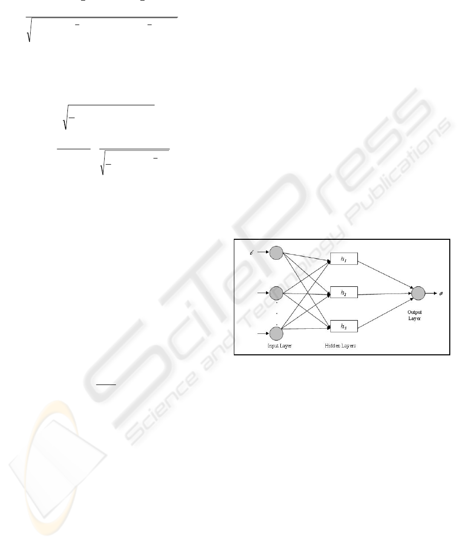
4.1.1 Model Description

The core architecture of the ANN was a feedforward

MLP (Figure 1) linking each input neuron with three

hidden layers, consisting of parallel slabs activated

by a different function (i.e., i-h

- h

– o, where

is the input vector h

, h

are the internal hidden

layers and o is the output). Variations of this

architecture were employed regarding the number of

inputs and the number of neurons in the internal

hidden layers, whereas the difference between the

actual and the predicted effort is manifested at the

output layer (forecasting deviation).

Figure 1: A Feed-forward MLP Neural Network.

Firstly, the ANN were trained in a supervised

manner, using the backpropagation algorithm. Also,

we utilised a technique to filter the data and reserve

holdout samples, namely training, validation and

testing subsets. The extraction was made randomly

using 70% of the data samples for training, 20% for

validation and 10% for testing. With

backpropagation the inputs propagate through the

ANN resulting in an output according to the initial

weights. The predicting behaviour of the ANN is

characterised by the difference among the predicted

and the desired output. Then, the difference is

propagated in a backward manner adjusting the

necessary weights of the internal neurons, so that the

predicted value is moved closer to the actual one in

the subsequent iteration. The training set is utilised

during the learning process, the validation set is used

to ensure that no overfitting occurs in the final result

ICEIS 2008 - International Conference on Enterprise Information Systems

and that the network is able to generalise the

knowledge gained. The testing set is an independent

dataset, i.e., does not participate during the learning

process and measures how well the network

performs with unknown data. During training the

inputs are presented to the network in patterns

(inputs/output) and corrections are made on the

weights of the network according to the overall error

in the output and the contribution of each node to

this error.

4.1.2 Results

The experiments conducted constituted an empirical

investigation mainly regarding the number of inputs

and internal neurons forming the layers of the ANN.

In these experiments several ANN parameters were

kept constant as some preliminary experiments

previously conducted implied that varying the type

of the activation function in each layer had no

significant effect on the forecasting quality. More

specifically, we employed the following functions:

for i the linear [-1,1], h

the Gaussian, h

the tanh, h

the Gaussian complement and for o the logistic

function. Also, the learning rate, the momentum, the

initial weights and the amount of iterations were set

to 0.1, 0.1, 0.3 and 10,000 respectively.

In addition, the randomly generated subsets were

given a specific chronological order (t

) and for each

repetition of the procedure a sliding window

technique was used to extract an input vector and

supply it to the ANN model. The window-sliding

size i varied, with i=1…5. Practically, this is

expressed in Table 1, covering the following Input

Output Methods (IOM):

(1-2) using the lines of code or the function points

of i projects we estimate the effort of the i-th

project;

(3-4) using lines of code or function points with

effort of the i-th project we estimate the effort

required for the next project (i+1)-th in the

series sequence;

(5-6) using lines of code or function points of the i-

th and (i+1)-th projects and effort of the i-th

project we estimate the effort required for the

(i+1)-th project.

Each input method may vary the number of past

samples per variable from 1 to 5 (i index).

Table 1: Sliding window technique to determine the ANN

input and output data supply method. (*where i=1…5).

Input

Output

Method

Inputs* Output*

IOM-1 LOC(t

) EFF(t

)

IOM-2 FP(t

) EFF(t

)

IOM-3 LOC(t

), EFF(t

) EFF(t

i+1

)

IOM-4 FP(t

), EFF(t

) EFF(t

i+1

)

IOM-5 LOC(t

), LOC(t

i+1

), EFF(t

) EFF(t

i+1

)

IOM-6 FP(t

), FP(t

i+1

), EFF(t

) EFF(t

i+1

)

The best results obtained utilising the ANN

model and various datasets are summarised in Table

2. The first column refers to the dataset used, the

second column to the input and output method

(IOM) with which i data inputs are fed to the model,

the third column refers to the ANN topology and the

rest of the columns refer to the error metrics during

the training and testing phase. The last two columns

indicate the number of predicted projects that have

the same sign tendency, in the sequence of the effort

samples and the total percentage of the successful

tendencies during testing. The figures in Table 2

show that an ANN model deploying a mixture of

architectures and input, output methods yields

various accuracy levels. More specifically, the

DESH`89 dataset achieves high prediction accuracy,

with lowest MRE equal to 0.05 and CC equal to 1.0.

The KEM`87 dataset also performs adequately well

with relatively low error figures. The worst

prediction performance is obtained with ALGAF`83

and COKEM`87 datasets. These failures may be

attributed to too few projects involved in the

prediction in the first case, and to the creation of a

heterogeneous dataset in the latter case. Finally, as

the results suggest, the COC`81 and KEM`87

datasets achieve adequately fit predictions and thus,

we may claim that the method is able to approximate

the actual development cost. Another observation is

that the majority of the best yielded results employ a

large number of internal neurons. Therefore, further

investigation is needed with respect to different

ANN topologies and IOM for the various datasets.

To this end we resorted to using a hybrid scheme,

combining ANN with GA, the latter attempting to

evolve the near to optimal network topology and

input/output schema that yields accurate predictions

and has reasonably small size (i.e., number of

neurons) so as to avoid overfitting.

4.2 A Hybrid Model Approach

The rationale behind this attempt was that the

performance of ANN highly depends on the size,

structure and connectivity of the network and results

SIZE AND EFFORT-BASED COMPUTATIONAL MODELS FOR SOFTWARE COST PREDICTION

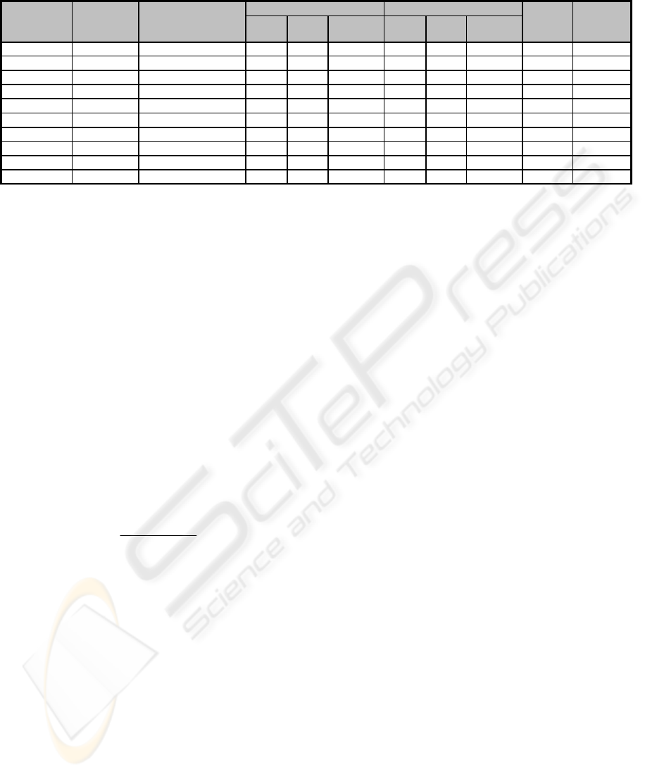
Table 2: Best Experimental Results obtained with the ANN-model.

DATASET

INPUT

OUTPUT

METHOD

ANN

ARCHITECTURE

TRAINING PHASE TESTING PHASE

Sign(p)

MRE CC NRMSE MRE CC NRMSE

COC`81 IOM-5 3-15-15-15-1 0.929 0.709 0.716 0.551 0.407 0.952 5/10 50.00

COC`81 IOM-1 2-9-9-9-1 0.871 0.696 0.718 0.525 0.447 0.963 7/12 58.33

KEM`87 IOM-1 1-15-15-15-1 0.494 0.759 0.774 0.256 0.878 0.830 2/3 66.67

KEM`87 IOM-5 5-20-20-20-1 0.759 0.939 0.384 0.232 0.988 0.503 2/2 100.00

COKEM`87 IOM-3 8-20-20-20-1 5.038 0.626 0.781 0.951 0.432 0.948 3/8 37.50

COKEM`87 IOM-3 4-3-3-3-1 5.052 0.610 0.796 0.768 0.257 1.177 4/8 50.00

ALGAF`83 IOM-6 5-3-3-3-1 0.371 0.873 0.527 1.142 0.817 0.649 3/4 75.00

ALGAF`83 IOM-2 2-20-20-20-1 0.335 0.975 0.231 1.640 0.936 0.415 2/4 50.00

DESH`89 IOM-4 4-9-9-9-1 0.298 0.935 0.355 0.481 0.970 0.247 17/20 85.00

DESH`89 IOM-4 6-9-9-9-1 0.031 0.999 0.042 0.051 1.000 0.032 20/20 100.00

may be further improved if the right parameters are

found. Therefore, we applied a GA to investigate

whether we can find the ideal network settings by

means of a cycle of generations including candidate

solutions that are pruned by the criterion ‘survival of

the fittest’, meaning the best performing ANN.

4.2.1 Model Description

The first task for producing the hybrid model was to

determine a type of encoding so as to express the

potential solutions (binary string representing the

ANN architecture, including inputs). The space of

all feasible solutions (the set of solutions among

which the desired solution resides) was called the

search space. Each point in the search space

represents one possible solution. Each possible

solution was “marked” by its fitness value, which in

our case was expressed in equation (7), minimizing

both the MRE and the size of the network.

ize

fitness

(7)

The GA looks for the best solution among a

number of possible solutions represented by one

point in the search space. Searching for a solution is

then equal to looking for some extreme value

(minimum or maximum) in the search space. The

GA developed included three types of operators:

selection (roulette wheel), crossover (with rate equal

to 0.25) and mutation (with rate equal to 0.01).

Selection chooses members from the population of

chromosomes proportionally to their fitness; and

also elitism was used to ensure that the best member

of each population was always selected for the new

population. Crossover adapts the genotype of two

parents by exchanging parts of them and creates a

new chromosome with a new genotype. Crossover

was performed by selecting a random gene along the

length of the chromosomes and swapping all the

genes after that point. Finally, the mutation operator

simply changes a specific gene of a selected

individual in order to create a new chromosome with

a different genotype.

4.2.2 Results

This section presents and discusses the results

obtained using the Hybrid model on the various

available datasets. The best ANN architectures

yielded are displayed in the third column of Table 3

with the various error figures obtained both during

the training and the testing phase.

The main observation is that for some of the

datasets the hybrid model optimised the ANN

prediction accuracy (i.e., ALGAF`83), whereas for

other datasets it performs adequately well in terms

of generalisation (i.e., DESH`89). More specifically,

the experiments show that the MRE is significantly

lowered during testing in almost all the datasets,

with KEM`87 being the only exception. The CC

improves or remains at the same levels in most of

the cases, whereas NRMSE deteriorates. The error

figures show that in most of the cases the yielded

architectures are consistent in that they improve the

respective estimations, even though the training

phase errors suggest that the ANN’s learning ability

is reduced. Another observation is that we cannot

suggest with confidence that this approach

universally improves the performance levels as the

yielded results are not consistent among the datasets,

even though the hybrid models manage to

generalise. It seems that while in some cases the

ANNs presented high learning success (e.g.,

DESH`89, ALGAF`83, KEM`87) in other cases

learning was quite poor (e.g., COC`81) as indicated

in the training phases. The results indicate that the

approach may be further improved, so that to

improve the learning ability of the ANNs and obtain

even better predictions.

ICEIS 2008 - International Conference on Enterprise Information Systems

Table 3: Hybrid model (coupling ANN and GA) results.

DATASET

INPUT OUTPUT

METHOD

YIELDED ANN

ARCHITECTURE

TRAINING PHASE TESTING PHASE

MRE CC NRMSE MRE CC NRMSE

COC`81 IOM-1 3-25-2-9-1

4.290 0.801 0.595

0.431

0.838 0.549

COC`81 IOM-3

2-16-21-18-1

6.356 0.736 0.668

1.967 0.942 0.556

COC`81 IOM-5 7-0-9-14-1 7.086 0.995 0.095 0.981 0.708 0.725

KEM`87 IOM-1 2-20-14-2-1 6.6445Ε-005 1.000 1.8165Ε-005 0.572 -0.552 1.521

KEM`87 IOM-3 2-11-4-5-1 4.5565Ε-006 1.000 1.735Ε-006 0.474 -0.500 1.593

KEM`87 IOM-5 5-6-19-6-1 3.4593Ε-006 1.000 7.0407Ε-007 0.572 -0.551 1.521

ALGAF`83 IOM-2 6-20-6-11-1 8.4427Ε-006 1.000 1.3176Ε-005 0.083 0.141 1.109

ALGAF`83 IOM-4 6-3-7-3-1 0.004 1.000 0.004 0.113 0.061 1.075

ALGAF`83 IOM-6 1-0-2-5-1 0.000 1.000 0.000 0.083 0.141 1.109

DESH`89 IOM-2 3-28-12-14-1 1.332 0.651 0.776 0.047 0.663 0.777

DESH`89 IOM-4 2-17-5-25-1 0.657 0.872 0.486 0.042 0.782 0.717

DESH`89 IOM-6 3-2-26-3-1 0.914 0.657 0.747 0.124 0.374 0.890

4.3 Comparison to a Classic

Regression-based Approach

In this section we present the results obtained from a

simple Multi-Linear Regression (MLR) model so as

to provide some comparative assessment of the

models proposed thus far. The MLR model will

assess how well the regression line approximates the

real effort and it is built with the leave-one-out

sampling testing technique. The assumption for this

model is that the dependent variable (effort) is

linearly related with the independent variable(s)

(size and/or next effort).

4.3.1 Model Description

The MLR model is built by employing the yielded b

coefficients from each of the IOM specified earlier

with the leave-one-out technique, both during

training and testing. According to equation (8) the

model produces the slope of a line that best fits the

data and then, during the testing phase we estimate

the value of the dependent variable using the sliding-

window. We assessed the values of the predicted and

actual effort calculated from the coefficients

influencing the independent variables of size and

effort in the regression equation with the

performance metrics.

exbxbby

+⋅

+⋅+= ...

110

(8)

4.3.2 Results

The MLR approach was tested only on the largest

datasets, namely COC`81 and DESH`89 which

yielded the best predictions with the ANN and thus a

comparison to the ANN models will become

feasible. The results of the MLR indicate average

performance for both datasets with precision

accuracy lower than the accuracy of both the

approaches proposed in this work (simple and hybrid

ANN). With the COC`81 dataset the yielded results

were MRE 3.017, CC 0.647 and NRMSE 0.798 for

the training, and 10.097, 0.011 and 3.029 for the

testing phase. With the DESH`89 dataset MRE was

equal to 1.035, CC 0.093, NRMSE 0.985 during

training and 1.57, 0.112 and 1.032 respectively

during testing. The main problem of the MLR

method yielding mediocre results may be attributed

mainly to the method’s dependence on the

distribution and normality of the data points used

and its inability to approximate unknown functions,

as opposed to the ability demonstrated by the ANN

and GA.

5 CONCLUSIONS

In the present work we attempted to study the

potentials of developing a software cost model using

computational intelligence techniques relying only

on size and effort project data. The core of the model

proposed consists of Artificial Neural Networks

(ANN) trained and tested using project size metrics

(Lines of Code, or, Function Points) and Effort,

aiming to predict the next project effort in the series

sequence as accurately as possible. Separate training

and testing subsets were used and serial sampling

with a sliding window propagated through the data

to extract the projects fed to the models. Commonly,

it is recognized that the yielded performance of an

ANN model mainly depends on the architecture and

parameter settings, and usually empirical rules are

used to determine these settings. The problem was

thus reduced to finding the ideal ANN architecture

for formulating a reliable prediction model. The first

experimental results indicated mediocre to high

prediction success according to the dataset used. In

addition, it became evident that there was need for

SIZE AND EFFORT-BASED COMPUTATIONAL MODELS FOR SOFTWARE COST PREDICTION

more extensive exploration of solutions in the search

space of various topologies and input methods as the

results obtained by the simple ANN model did not

converge to a general solution. Therefore, in order to

select a more suitable ANN architecture, we resorted

to using Evolutionary Algorithms. More specifically,

a Hybrid model was introduced consisting of ANN

and Genetic Algorithms (GA). The latter evolved a

population of networks to select the optimal

architecture and inputs that provided the most

accurate software cost predictions. In addition, a

classic MLR model was utilised as benchmark so as

to perform comparison of the results.

Although the results of this work are at a

preliminary stage it became evident that the ANN

approach combined with a GA yields better

estimates than the MLR model and that the

technique is very promising. The main limitation of

this method, as well as any other size-based

approach, is that size estimates must be known in

advance to provide accurate enough effort

estimations, and, in addition, there is a large

discrepancy between the actual and estimated size,

especially when the estimation is made in the early

project phases. Finally, the lack of a satisfactory

volume of homogeneous data as well as of definition

and measurement rules for size units such as LOC

and FP result in uncertainty to the estimation

process. The software size is also affected by other

factors that are not investigated by the models, such

as programming language and platform, and in this

work we emphasised only on coding effort which

accounts for only a percentage of the total effort in

software development. Another important limitation

with the technologies used is that the ANNs are

considered “black boxes” and the GA requires

extensive space search which is very time-

consuming. Therefore, future research steps will

concentrate on ways to improve performance;

examples of which may be: (i) study of other factors

affecting development effort and their

interdependencies, (ii) further adjustment of the

ANN and GA parameter settings, such as

modification of the fitness function, (iii)

improvement of the efficiency of the algorithms by

testing more homogeneous or clustered data and,

(iv) improvement of the quality of the data and use

more recent datasets to achieve better convergence.

REFERENCES

Albrecht, A.J., 1979. Measuring Application Development

Productivity, Proceedings of the Joint SHARE,

GUIDE, and IBM Application Developments

Symposium, pp.83-92.

Albrecht, A.J. and Gaffney J.R., 1983. Software Function

Source Lines of Code, and Development Effort

Prediction: A Software Science Validation, IEEE

Transactions on Software Engineering, 9(6), pp. 639-

648.

Boehm, B.W., 1981. Software Engineering Economics.

Prentice Hall.

Boehm, B.W., Abts, C., Clark, B., and Devnani-Chulani.

S., 1997. COCOMO II Model Definition Manual. The

University of Southern California.

Briand L. C. and Wieczorek I., 2001. Resource Modeling

in Software Engineering, Encyclopedia of Software

Engineering 2.

Burgess, C. J. and Leftley M., 2001. Can Genetic

Programming Improve Software Effort Estimation? A

Comparative Evaluation, Information and Software

Technology, 43 (14), Elsevier, Amsterdam, pp. 863-

873.

Charette, R. N., 2005. Why software fails, Spectrum IEEE

42 (9), pp. 42-29.

Desharnais, J. M., 1988. Analyse Statistique de la

Productivite des Projects de Development en

Informatique a Partir de la Technique de Points de

Fonction. MSc. Thesis, Montréal (Université du

Québec).

Dolado, J. J., 2001. On the Problem of the Software Cost

Function, Information and Software Technology, 43

(1), Elsevier, pp. 61-72.

Fenton, N.E. and Pfleeger, S.L., 1997. Software Metrics: A

Rigorous and Practical Approach. International

Thomson Computer Press.

Haykin, S., 1999. Neural Networks: A Comprehensive

Foundation, Prentice Hall.

Jorgensen, M., and Shepperd M., 2007. A Systematic

Review of Software Development Cost Estimation

Studies. Software Engineering, IEEE Transactions on

Software Engineering, 33(1), pp. 33-53.

Kemerer, C. F., 1987. An Empirical Validation of

Software Cost Estimation Models, CACM, 30(5), pp.

416-429.

Park, R., 1996. Software size measurement: a framework

for counting source statements, CMU/SEI-TR-020.

Available:http://www.sei.cmu.edu/pub/documents/92.r

eports/pdf/tr20.92.pdf, Accessed Nov, 2007.

Software Magazine, 2004. Standish: Project success rates

improved over 10 years.

Available:http://www.softwaremag.com/L.cfm?Doc=n

ewsletter/2004-01-15/Standish, Accessed Nov, 2007.

Sommerville, I., 2007. Software Engineering, Addison-

Wesley.

Wittig, G. and Finnie G., 1997. Estimating software

development effort with connectionist model.

Information and Software Technology, 39, pp.469-

476.

ICEIS 2008 - International Conference on Enterprise Information Systems