D
YNAMIC SEMI-MARKOVIAN WORKLOAD MODELING
Nima Sharifimehr and Samira Sadaoui
Department of Computer Science, University of Regina, Regina, Canada
Keywords:
Markovian Models, Workload Modeling, Enterprise Application Servers.
Abstract:
In this paper, we present a Markovian modeling approach which is based on a combination of existing Semi-
Markov and Dynamic Markov models. The proposed approach is designed to be an efficient statistical
modeling tool to capture both actions intervals patterns and sequential behavioral patterns. A formal defi-
nition of this model and detailed algorithms for its implementation are illustrated. We show the applicability
of our approach to model workload of enterprise application servers. However, the given formal definition
of our proposed approach prepares a firm ground for academic researchers to investigate many other possible
applications. Finally, we prove the accuracy of our dynamic semi-Markovian approach for the most chaotic
situations.
1 INTRODUCTION
The performance of software systems is significantly
affected by the incoming workload toward them (Ro-
lia et al., 2006). To improve the performance of
such systems, we need to analyze the workload they
process. Through workload modeling, we can find
the bottlenecks and issues which reduce the through-
put of software systems. However, analyzing real
workload is an extremely difficult task and on the
other hand reproducing workload with specific fea-
tures is not easily feasible (R.J. Honicky and Sawyer,
2005). Using modeling approaches to build a generic
workload model for a given system is an appropriate
solution to control the complexity of workload analy-
sis. Markovian models have been widely used for the
purpose of modeling workload processed by software
systems (Dhyani et al., 2003) (Eirinaki et al., 2005)
(Sarukkai, 2000). Also some combinatory approaches
have been investigated, which take advantage of com-
bining Markovian models with other techniques such
as clustering (F. Khalil and Wang, 2007), and neural
networks (Firoiu and Cohen, 2002).
In this paper we are interested in workload
modeling for enterprise application servers. Enter-
prise application servers as server programs in dis-
tributed infrastructures provide development and de-
ployment facilities to integrate all organizations’ ap-
plications and back-end systems (Mariucci, 2000).
We view the workload modeling as the process of ana-
lyzing the sequence of incoming requests and finding
patterns across method invocations on hosted applica-
tions and components. Investigated approaches in the
literature on workload modeling only focus on extrac-
tion of sequential patterns of incoming requests. They
do not discuss solutions for capturing patterns of in-
tervals between incoming requests and their process
times. Therefore, in this paper we illustrate a Dy-
namic Semi-Markov Model (DSMM) which can be
used to efficiently model the incoming workload to-
ward an enterprise application server. Our modeling
approach enhances current Markov modeling solu-
tions (R.J. Honicky and Sawyer, 2005) (Song et al.,
2004) for accurate workload modeling. DSMM cap-
tures patterns of intervals between incoming requests,
the required times to process them, and also their
sequential model. In other words, it finds patterns
across incoming requests and also statistical models
of requests intervals and process times. Measuring
the accuracy of our proposed approach for the most
chaotic situations, we show that DSMM-based work-
load modeling for enterprise application servers is a
very accurate solution.
The rest of this paper is structured as follows. Sec-
tion 2 introduces our dynamic-semi Markov Model.
Section 3 explains the dynamic building process to
build and adjust a DSMM. Section 4 illustrates the re-
sults of experimentations that evaluate the accuracy of
125
Sharifimehr N. and Sadaoui S. (2008).
DYNAMIC SEMI-MARKOVIAN WORKLOAD MODELING.
In Proceedings of the Tenth International Conference on Enterprise Information Systems - DISI, pages 125-130
DOI: 10.5220/0001678801250130
Copyright
c
 SciTePress

DSMMs. Finally, Section 5 concludes the paper with
some future directions.
2 DYNAMIC SEMI-MARKOV
MODEL
This section introduces a Dynamic Semi-Markov
Model (DSMM) which dynamically adapts itself to
the analyzing data. DSMM is designed with this
goal in mind to be an accurate and efficient work-
load modeling tool for enterprise application servers.
A DSMM is a Kripkle or temporal structure (van der
Hoek et al., 2005) in which transitions and states are
labeled with probability distributions. The probabil-
ity distributions attached to a transition describe the
speed of evolution from one state to another and also
the probability of the occurrence of that transition
in terms of discrete distribution functions (Zellner,
2004). The probability distribution attached to a state
is also a discrete distribution function but it describes
the idle time spent when a transition evolves the sys-
tem to a new state. Consequently, being a change in
the system - a transition from the current state to an-
other - depends on the attached time distribution func-
tions to states and transitions. This dependency which
is in contradiction with Markov property (Cover and
Thomas, 2006) makes DSMM a semi-Markov (L
´
opez
et al., 2001) rather than Markov. In the following
comes the formal definition of DSMM.
Definition 1. (Dynamic Semi-Markov Model)
Let AP be a finite set of tokens seen in
the analyzing data. A DSMM is a 5-tuple
(S, T, P, PDF
S
, PDF
T
) where:
• S is a finite set of states.
• T is a finite set of discrete time units [t
min
,t
max
].
• P: S × AP → S × [0,1] is the transition function
which states the probability of evolving the sys-
tem from a state to another when a specific ele-
ment is seen in the analyzing data.
• PDF
S
: S × T → [0,1] is the idle time probabil-
ity matrix (satisfying
∑
t∈T
PDF
S
(s,t) = 1 for each
s ∈ S ).
• PDF
T
: S × AP × T → [0, 1] is the probability ma-
trix (satisfying
∑
t∈T
PDF
T
(s,a,t) = 1 for each
s ∈ S and a ∈ AP ) for the evolution speed of the
system when a specific element is seen in the an-
alyzing data.
Figure 1 shows an example of DSMM which only
contains two states of S
0
and S
1
and the tokens of the
analyzing data belongs to the finite set of {0,1}.
Figure 1: An example of DSMM.
3 DYNAMIC PROCESS OF
BUILDING A DSMM
The formal definition of DSMM mentioned above de-
scribes the static structure of a DSMM and the exam-
ple shown afterward illustrates how a typical DSMM
looks like at a time snapshot of its lifecycle. How-
ever, one significant aspect of a DSMM is its dynamic
nature. A DSMM changes dynamically during its life-
cycle to find the best fit model for a specific system.
Dynamic process of building a DSMM brings two sig-
nificant advantages:
• When all or some internal states of a system are
unknown, this dynamic building process starts
building the DSMM with only one state and then
extracts the others through the statistical analy-
sis of the processing data. This speeds up the
modeling process and makes it possible to easily
model systems with unperceivable internal states.
• A DSMM is useful even before being close
enough to the best fit model. In other words, a
DSMM can be used during the dynamic building
process when it is not as accurate as final built
model. This feature is so critical for real-time sys-
tems where late results of a process are considered
incorrect (Shaw, 2000).
Before giving a formal definition for the best fit
model, an accuracy measurement tool is required. For
this sake, it is shown how to measure Root Mean
Square Error (RMSE) (Zellner, 2004) of a DSMM
based on a stream of sample data taken from the
modeling system.
3.1 Rmse of a DSMM
Let assume a stream of analyzing data from a specific
system is described as a finite sequence of 3-tuples
(I
0
,A
0
,E
0
) → ... → (I
i
,A
i
,E
i
) → ... → (I
n
,A
n
,E
n
)
where I
i
shows the idle time before the observation of
the next token in the stream of analyzing data, A
i
is the
ICEIS 2008 - International Conference on Enterprise Information Systems
126

next token which system emits after spending the idle
time, and E
i
is the evolution speed which describes
the time that system spends to emit A
i
. Processing the
tuples of this sequence through the steps mentioned
below generates a prediction sequence which will be
used directly to compute the RMSE of a model:
Algorithm 1. Prediction Sequence Generation
1. Define S as a state
2. S ← Starting state of DSMM
3. j ← 0
4. For each i ∈ [0,n]
(a) Define P
j
t
, P
j+1
t
, P
j+2
t
as probabilities
(b) P
j
t
← PDF
S
(S,I
i
)
(c) P
j+1
t
← P(S,A
i
)
(d) P
j+2
t
← PDF
T
(S,A
i
,E
i
)
(e) Add P
j
t
, P
j+1
t
, and P
j+2
t
to the prediction se-
quence
(f) S ← P(S,A
i
)
(g) j ← j + 3
Subsequently using the resulted prediction sequence
generated through Algorithm 1, RMSE of a model can
be computed through the following formula (Zellner,
2004):
RMSE =
s
∑
n∗3
i=0
(P
i
t
− 1)
2
n ∗ 3
Following comes the formal definition of the best
fit model which defines the ideal goal of building a
DSMM.
Definition 2. (The Best Fit Model)
A DSMM is the best fit model of a specific system
when its RMSE for any sample data from that system
equals to zero.
However, building the best fit models in the real
world is almost impossible in most cases. Therefore,
the ideal goal of modeling a system can be stated as
building the closest model to the best fit model. In
other words, the modeling process aims to reduce the
RMSE of a model as much as possible.
3.2 Building a DSMM
Having the formal definition of the ideal goal for
modeling a system, it is time to dig into the dynamic
process of building a model. Algorithm 2 used for this
purpose is based on the dynamic modeling approach
used in Dynamic Markov Compression (DMC) (Or-
mack and Horspool, 1987). Also the applicability and
efficiency of this modeling approach has been proven
before on workload modeling with the purpose of de-
veloping a predictive automatic tuning service for ob-
ject pools (Sharifimehr and Sadaoui, 2007). Though
it is heavily modified to be applicable for the semi-
Markov model proposed above. Basically the algo-
rithm starts with a DSMM which only contains one
state S
0
and this starting DSMM can be illustrated as
follows (let assume AP = {a,b}) :
• P
1
t
= PDF
S
(S
0
,t) where PDF
S
(S
0
,t) is a uniform
discrete distribution, so we can say for all values
of t ∈ T we have PDF
S
(S
0
,t) = 1/(t
max
− t
min
)
which also satisfies
∑
t
max
t=t
min
PDF
S
(S
0
,t) = 1.
• P(S
0
,a) = P(S
0
,b) = (S
0
,0.5) which states that
the observation of all allowed tokens (i.e. a and
b) in the analyzing data evolves the system back
to S
0
and the probability of observation of each is
equal.
• P
2
t
= PDF
T
(S
0
,a,t) and P
3
t
= PDF
T
(S
0
,b,t)
where both of them are again uniform discrete
distributions, so we have PDF
T
(S
0
,a,t) =
PDF
T
(S
0
,b,t) = 1/(t
max
− t
min
) and also
∑
t
max
t=t
min
PDF
T
(S
0
,a,t) =
∑
t
max
t=t
min
PDF
T
(S
0
,b,t) =
1.
Subsequently we set the only state of DSMM men-
tioned above as the current state, namely S
C
. Then
for each 3-tuple i.e. (I
i
,A
i
,E
i
) in the analyzing data,
we go through the steps of Algorithm 2 , mentioned
below. Algorithm 2 dynamically evolves the DSMM
into a model closer to the best fit model.
Algorithm 2. Building a DSMM Dynamically
1. Update the idle time distribution of the current
state based on the idle time I
i
. To store idle time
distributions, each DSMM uses a two dimensional
array: IDLE[S
0
..S
MAX
][t
min
..t
max
]. Consequently,
to figure out the probability of spending t
i
time
units in state S
C
, the following formula can be
used:
PDF
S
(S
C
,t
i
) = IDLE[S
C
][t
i
]/
∑
t
max
t=t
min
IDLE[S
C
][t]
So, to update the idle time distribution of state S
C
when the idle time I
i
is in the current processing
3-tuple of the analyzing data, we need to only per-
form the following operation:
IDLE[S
C
][t
i
] ← IDLE[S
C
][t
i
] + 1
2. Update the transition time distribution of the tran-
sition which evolves the system to its next new
state based on the observation of A
i
which takes
E
i
time duration. A three dimensional array
SPEED[S
0
..S
MAX
][A
0
..A
|AP|
][t
min
..t
max
] is used to
store transition time distributions for each DSMM.
Therefore, to compute the probability of evolving
DYNAMIC SEMI-MARKOVIAN WORKLOAD MODELING
127

from state S
C
after the observation of A
i
within E
i
time, we have:
PDF
T
(S
C
,A
i
,E
i
) =
SPEED[S
C
][A
i
][E
i
]/
∑
t
max
t=t
min
SPEED[S
C
][A
i
][t]
So, to update the transition time distribution of
evolution from the current state S
C
with observa-
tion of A
i
when the transition time E
i
is in the cur-
rent processing 3-tuple of the analyzing data, we
need to only perform the following operation:
SPEED[S
C
][A
i
][E
i
] ← SPEED[S
C
][A
i
][E
i
] + 1
3. Update the transition probability of evolving from
the current state as a result of the observation of
A
i
. For this sake, there is a couple of two dimen-
sional arrays: MOV E[S
0
..S
MAX
][A
0
..A
|AP|
] and
COUNT [S
0
..S
MAX
][A
0
..A
|AP|
] attached to each
DSMM. The array MOV E shows which state the
system evolves to from each state after the obser-
vation of each token and the array COUNT keeps
track of the number of times each token has been
observed in each state of the model. These two
arrays are the building elements of the transition
function P:
P(S
C
,A
i
) = (MOV E[S
C
][A
i
] ,
COUNT [S
C
][A
i
]/
∑
a∈AP
COUNT [S
C
][a])
Then updating the transition probability of evolv-
ing from the current state after the observation of
A
i
is done by:
COUNT [S
C
][A
i
] ← COUNT [S
C
][A
i
] + 1
4. If it is suitable add a new state(s) to the model to
reduce its RMSE and afterwards adjust involved
parameters of the model. Adding a new state to
the model which we refer to as cloning is an effec-
tive way to improve its fitness. The idea is when
transition to the state S
N
= MOV E[S
C
][A
i
] from
the current state S
C
is more probable than any
other state, we clone the state S
N
to capture more
details about that specific evolution in the system.
We can use the cloning conditions proposed in
DMC (Ormack and Horspool, 1987) and adapt it
to the definition of DSMM. So when the following
conditions are satisfied cloning happens:
(a) T hreshold
1
≤ COUNT [S
C
][A
i
]
(b) T hreshold
2
≤
∑
a∈AP
COUNT [S
N
][a] −
∑
a∈AP
COUNT [S
C
][a]
First condition is to make sure the transition from
S
C
to S
N
has taken enough times (i.e. more than
T hreshold
1
times). And the second condition is
to assure that transitions to S
N
from S
C
is more
probable than any other state and T hreshold
2
is
used to describe this condition.
5. Change the current state of the model according to
the observed token A
i
. Having the array MOV E as
explained above based on the observation A
i
, this
change of state is carried out as follows:
S
C
← MOV E[S
C
][A
i
]
3.3 Adjustment of Parameters
To model real-world systems accurately and effi-
ciently using DSMMs, we need to take the follow-
ing points into account when adjusting parameters of
Algorithm 2 proposed above (Ormack and Horspool,
1987):
• Choosing small values for Threshold
1
and
T hreshold
2
will increase the growth speed of the
model. In contrast, assigning large values to
these parameters decrease the speed of adding
new states to the model. Adding more states to the
model helps to capture more details about the be-
havior of the system. However, it does not mean
necessarily that the model will get closer to the
best fit model faster. Unfortunately there are no
absolute values for these parameters which can be
used to model all systems. An applicable way
is to find their values specifically for each sys-
tem through a feed-back based approach. A typ-
ical feed-back based solution measures the accu-
racy of the model actively and whenever the ac-
curacy is not showing any change, the values of
T hreshold
1
and T hreshold
2
will be reduced.
• Adjusting the maximum number of states, namely
MAX
S
, depends on available memory accessible
to the modeling process. However, an issue which
should be addressed is how to react when the
number of states in a model reaches this max-
imum. Dynamic Markov Compression (DMC)
(Ormack and Horspool, 1987) suggests to discard
the model and start the modeling process from
the scratch again. Though this approach is use-
ful when the modeled behavior is not going to be
used in the future. Otherwise, we can save the cur-
rent model into a persistent storage and then start
with a new model.
4 EVALUATION RESULTS
We conduct our experimentations using synthetic
workload models defined by RUBiS (Cecchet et al.,
2002) to evaluate the accuracy of the proposed ap-
proach for workload modeling using DSMMs. These
workload models are designed according to standards
introduced in TPC-W (Garcia and Garcia, 2003)
ICEIS 2008 - International Conference on Enterprise Information Systems
128

which model an online bookstore (see clauses 5.3.1.1.
and 6.2.1.2 of the TPC-W v1.6 specification (Council,
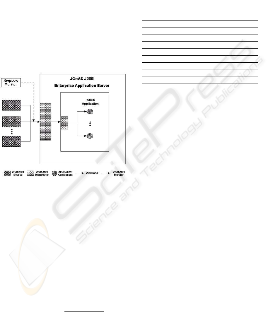
2001)). For this purpose, we use JOnAS J2EE (Sicard
et al., 2006) as our enterprise application server and
integrate an incoming request monitor into it as is
shown in Figure 2. We use a machine equipped with
PIV 2.80 GHz CPU, 1 GB of RAM. Also we use
MSSQL Server 2000 as the backend DBMS running
on MS Windows Server 2003 Service Pack 1. In this
architecture, we use RUBiS client module to simu-
late our workload generators. The RUBiS client mod-
ule generates workloads with high randomness which
simulates the most chaotic situation. Therefore, the
results of our experimentations show the accuracy of
DSMMs for the worst case scenarios.
Figure 2: Integration of an incoming requests monitor into
JOnAS J2EE which hosts RUBiS application.
Algorithm 2 is only capable of processing a sequence
of 3-tuples (I
0
,A
0
,E
0
) → .. → (I
i
,A
i
,E
i
) → ... →
(I
n
,A
n
,E
n
). Therefore, we implement a converter
module which is responsible for generating this se-
quence from a monitored workload.
To evaluate the accuracy of our approach which is
based on DSMM, we use sample data tracing. For
this purpose, at first we build a DSMM for work-
load generated by RUBiS clients according to a spe-
cific workload model. Afterward, we generate an-
other sequence of workload based on the same work-
load model and trace it on the built DSMM. The
tracing process will generate a sequence of 3-tuples
(P
0
I
,P
0
A
,P
0
E
) → ... → (P
i
I
,P
i
A
,P
i
E
) → ... → (P
n
I
,P
n
A
,P
n
E
).
Then the average difference between the DSMM and
real workload model can be measured as follows:
di f f erence =
∑
n
i=0
(1−P
i
I
)+(1−P
i
A
)+(1−P
i
E
)
3
n
And as the similarity between the DSMM and the real
workload equals to the complement of the average
difference, we have:
similarity = 1 − di f f erence
Table 1: Similarity of built DSMMs and real workloads.
Workload MAX
S
MAX
S
MAX
S
MAX
S
= 10 = 50 = 100 = 500
W0 0.36 0.45 0.45 0.49
W1 0.37 0.41 0.45 0.49
W2 0.37 0.44 0.45 0.49
W3 0.34 0.43 0.46 0.50
W4 0.36 0.44 0.46 0.49
W5 0.34 0.42 0.47 0.48
W6 0.36 0.41 0.45 0.49
W7 0.37 0.43 0.46 0.49
W8 0.37 0.42 0.42 0.49
W9 0.35 0.45 0.45 0.49
Table. 1 shows the resulted similarity of built DSMMs
for each generated workload i.e. W
i
. It also illus-
trates the relationship between size of DSMMs and
their measured similarity for different workloads.
Interestingly, increasing the size of a DSMM in-
creases the similarity only for a while. In other words,
the accuracy of a DSMM becomes stable after a spe-
cific size and does not increase anymore. These re-
sults show that DSMM-based workload modeling can
reach the accuracy of approximately 50% in the most
chaotic situation which the incoming workload has
high randomness. Therefore, our proposed approach
based on DSMM is an efficient and accurate workload
modeling solution for enterprise application servers.
5 CONCLUSIONS
In this paper, we have introduced a dynamic semi-
Markovian approach to model the incoming workload
toward an Enterprise Application Server. DSMM is
designed to be an efficient workload modeling tool for
enterprise application servers. A formal definition of
the DSMM independent of its proposed application in
this paper is given. This formal definition allows other
researchers to investigate other possible applications
of DSMM.
Afterwards, step by step procedure of building a
DSMM for a typical system is illustrated. The brief
explanation of this procedure assures that sufficient
information is provided for real-world applications.
Also to make the DSMM useful for a wide range
of applications, adjustment techniques has been dis-
cussed.
Finally, to prove the accuracy of the proposed ap-
proach for the real-world applications, experiments
DYNAMIC SEMI-MARKOVIAN WORKLOAD MODELING
129

for the most chaotic situations are carried out. The
result of experiments show that DSMM-based work-
load modeling for enterprise application servers is a
very accurate solution.
REFERENCES
Cecchet, E., Marguerite, J., and Zwaenepoel, W. (2002).
Performance and scalability of ejb applications. In
OOPSLA ’02: Proceedings of the 17th ACM SIG-
PLAN conference on Object-oriented programming,
systems, languages, and applications, pages 246–261,
New York, NY, USA. ACM Press.
Council, T. P. P. (2001). TPC Benchmark W, Standard Spec-
ification.
Cover, T. M. and Thomas, J. A. (2006). Elements of Infor-
mation Theory (Wiley Series in Telecommunications
and Signal Processing). Wiley-Interscience.
Dhyani, D., Bhowmick, S. S., and Ng, W.-K. (2003). Mod-
elling and predicting web page accesses using markov
processes. In DEXA ’03: Proceedings of the 14th
International Workshop on Database and Expert Sys-
tems Applications, page 332, Washington, DC, USA.
IEEE Computer Society.
Eirinaki, M., Vazirgiannis, M., and Kapogiannis, D. (2005).
Web path recommendations based on page ranking
and markov models. In WIDM ’05: Proceedings of
the 7th annual ACM international workshop on Web
information and data management, pages 2–9, New
York, NY, USA. ACM.
F. Khalil, J. L. and Wang, H. (2007). Integrating markov
model with clustering for predicting web page ac-
cesses. In AusWeb’07: Proceedings of the 13th Aus-
tralian World Wide Web conference, Australia.
Firoiu, L. and Cohen, P. R. (2002). Segmenting time se-
ries with a hybrid neural networks - hidden markov
model. In Eighteenth national conference on Artificial
intelligence, pages 247–252, Menlo Park, CA, USA.
American Association for Artificial Intelligence.
Garcia, D. F. and Garcia, J. (2003). Tpc-w e-commerce
benchmark evaluation. Computer, 36(2):42–48.
L
´
opez, G. G. I., Hermanns, H., and Katoen, J.-P. (2001).
Beyond memoryless distributions: Model checking
semi-markov chains. In PAPM-PROBMIV ’01: Pro-
ceedings of the Joint International Workshop on Pro-
cess Algebra and Probabilistic Methods, Performance
Modeling and Verification, pages 57–70, London, UK.
Springer-Verlag.
Mariucci, M. (2000). Enterprise application server devel-
opment environments. Technical report, Institute of
Parallel and Distributed High Performance Systems.
Mosbah, M. and Saheb, N. (1997). A syntactic approach to
random walks on graphs. In WG ’97: Proceedings of
the 23rd International Workshop on Graph-Theoretic
Concepts in Computer Science, pages 258–272, Lon-
don, UK. Springer-Verlag.
Ormack, G. V. and Horspool, R. N. S. (1987). Data com-
pression using dynamic markov modelling. Comput.
J., 30(6):541–550.
R.J. Honicky, S. R. and Sawyer, D. (2005). Workload
modeling of stateful protocols using hmms. In pro-
ceedings of the 31st annual International Conference
for the Resource Management and Performance Eval-
uation of Enterprise Computing Systems, Orlando,
Florida.
Rolia, J., Cherkasova, L., and Friedrich, R. (2006). Per-
formance engineering for enterprise software systems
in next generation data centres. Technical report, HP
Laboratories.
Sarukkai, R. R. (2000). Link prediction and path analy-
sis using markov chains. Comput. Networks, 33(1-
6):377–386.
Sharifimehr, N. and Sadaoui, S. (2007). A predictive auto-
matic tuning service for object pooling based on dy-
namic markov modeling. In Proc. of 2nd Interna-
tional Conference on Software and Data Technolo-
gies, Barcelona, Spain.
Shaw, A. C. (2000). Real-Time Systems and Software. John
Wiley & Sons, Inc., New York, NY, USA.
Sicard, S., Palma, N. D., and Hagimont, D. (2006). J2ee
server scalability through ejb replication. In SAC
’06: Proceedings of the 2006 ACM symposium on
Applied computing, pages 778–785, New York, NY,
USA. ACM.
Song, B., Ernemann, C., and Yahyapour, R. (2004). Paral-
lel computer workload modeling with markov chains.
In Job Scheduling Strategies for Parallel Processing,
pages 47–62, London, UK. Springer Verlag LNCS.
van der Hoek, W., Jamroga, W., and Wooldridge, M. (2005).
A logic for strategic reasoning. In AAMAS ’05: Pro-
ceedings of the fourth international joint conference
on Autonomous agents and multiagent systems, pages
157–164, New York, NY, USA. ACM Press.
Vose, M. D. (1991). A linear algorithm for generating ran-
dom numbers with a given distribution. IEEE Trans.
Softw. Eng., 17(9):972–975.
Zellner, A. (2004). Statistics, Econometrics and Forecast-
ing. Cambridge University Press.
ICEIS 2008 - International Conference on Enterprise Information Systems
130