VARIABILITY MANAGEMENT IN SOFTWARE PRODUCT

LINES FOR DECISION SUPPORT SYSTEMS CONSTRUCTION

María Eugenia Cabello and Isidro Ramos

Polytechnic University of Valencia,Camino de Vera s/n, 46022 Valencia, Spain

Keywords: Software Product Lines, Decision Support Systems, Variability Management, Software Architectures.

Abstract: This paper presents software variability management in complex cases of Software Product Lines where

two kinds of variabilities emerge: domain variability and application variability. We illustrate the problem

by means of a case study in Decision Support Systems. We have death with the first one by using variability

points that are captured using decision-tree techniques in order to select base architectures and the second

one by decorating the base architectures with the features of the application domain. In order to present this

variability management, we focus on the diagnostic domain, a special case of Decision Support Systems. A

generic solution for the automatic construction of systems of this kind is given using our approach: Baseline

Oriented Modeling (BOM).

1 INTRODUCTION

The development of Decision Support Systems is

complex since the elements that form their software

architecture vary. These architectural elements

change in their behaviour and in their structure.

In these kinds of systems, the variability

management cannot be performed through a unique

Feature Model, and the variability must be treated in

two phases: the first phase through different base

architectures derived from a unique generic

architecture; and the second phase by means of a

more classic treatment using a Feature Model and

decorating these base architectures with different

features.

We have illustrated the variability management

in the domain of Decision-Oriented Systems, and an

application field: the diagnosis of educational

programs using BOM (Baseline Oriented Modeling).

BOM is a framework that semi-automatically

generates DSS in a particular domain, based on

product lines techniques.

Our work integrates different technological

spaces to cope with the complexity of the problem.

These are the following: a) The generic architecture

of Decision Support Systems (DSS) (Turban et al.,

2001) to capture the knowledge of experts and to try

to imitate their reasoning processes when they solve

problems in a certain domain; b) Model-Driven

Architecture (MDA of OMG) (http://www.org/mda)

at the abstract modelling level (PIM); c) The

PRISMA Architectural Framework (Pérez, 2006) as

the target software level (PSM); d) The Software

Product Lines (SPL) (Clements et al., 2002) as a

technique for systematic reuse in software products,

and e) Feature-Oriented Modeling (FOM) (Trujillo,

2007) to capture the different variabilities of the

problem.

Several methodologies and applications on SPL

have produced a wide variety of research products,

offering suggestions and solutions in specific

domains. Our research is related to the following

works:

i) (Batory et al.,2006) express the domain

features in the Feature Model.

ii) (Trujillo, 2007) uses Feature-Oriented

Programming as a technique for inserting

the features.

iii) (González-Braixauli et al.,2005) apply the

MDA proposal as well as Requirements

Engineering for Product Lines.

iv) (Clements et al., 2002) use the SPL

development approach, considering a

division between domain engineering and

application engineering phases for the reuse

and the automation of the software process.

v) (Trujillo, 2007) has developed the XAK

tool for inserting features into XML

documents by means of XSLT templates.

Eugenia Cabello M. and Ramos I. (2008).

VARIABILITY MANAGEMENT IN SOFTWARE PRODUCT LINES FOR DECISION SUPPORT SYSTEMS CONSTRUCTION.

In Proceedings of the Tenth International Conference on Enterprise Information Systems - ISAS, pages 49-56

DOI: 10.5220/0001675300490056

 SciTePress

vi) (Santos, 2005) proposes the development of

a technique based on MDA for variability

management in Software Product Lines.

vii) The AMPLE project (http://www.ample-

project.net) deals with variability

management in different ways. This project

mentions that (Bachman et al., 2005)

propose to separate the variability

declaration from the affected artifacts.

The structure of the paper is the following: Section 2

presents the variability management in the DSS.

Section 3 introduces the variability dimensions of

our domain (diagnosis). Section 4 introduces the

variability in the application domain. Section 5

describes the design of the Decision Software

Architecture. Section 6 presents our conclusions and

provides some ideas for future work.

2 VARIABILITY MANAGEMENT

IN DECISION SUPPORT

SYSTEMS

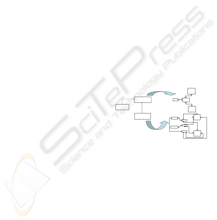
The development process of a specific application

(member of the product line) starts from a unique

generic architecture of the domain. The DSS domain

unique generic architecture is presented in Figure

1(a). This implies the existence of additional

particular features that are represented as variability

points, and their choice configure the final product.

However, another variability emerges, in complex

application domains. This variability is represented

by the existence of several base architectures for the

same generic architecture (see Figure 1(b)). We use

a Modular view for describing the generic

architecture conforming a Modular view metamodel

(MM MODULAR VIEW) and a Component-

Connector view for describing the Base

Architectures Skeletons conforming a Component-

Connector view metamodel (MM C-C

SKELETON). Figure 1 shows a unique generic

architecture and two base architectures.

In these cases, there are two variability types

which are orthogonal: one provided by the domain

(e.g. diagnosis) and another one provided by the

application domain (e.g. medical diagnosis,

educational diagnosis).

Therefore, we have treated variability in two

phases. The initial variability is treated through

variability points in a Decision Tree (DT). This DT

selects the right base architecture. The second

variability is managed by decorating this base

architecture with the features of the application

domain.

To illustrate our approach, we have selected a

case study: the diagnosis of educational programs

within the diagnosis domain. Our research considers

the following ontology:

• The diagnosis consists of interpreting the status

of an entity through its properties.

• In the application domain of the diagnosis, the

entity to be diagnosed is a postgraduate

academic program, and the diagnosis result is

the level of development of this program. The

properties of the entities belong to the features

and sub-features that are evaluated to obtain the

validation of only one hypothesis

(appropriate/inappropriate) as a result of the

diagnosis.

• The scenario for the academic diagnosis process

is as follows: the system takes data that are

given as input by the final user and relates it to

the features of the educational program. The

system infers other properties by deduction and

subsequently does the same for the hypothesis.

The result is the development level of the

educational program.

INFERENCE

PROCES S

KNOWLEDGE

BASE

USER

DIAGNOSTIC

CONNECTOR

INFERENCE

PROCESS

KNOWLEDGE

BASE

CLINICAL

USER

LABORATORY

USER

Connector 1

Connector 2

Connector 3

INFERENCE PROCESS

KNOWLEDGE BASE

USER INTERFACE

(a) Modular View (b) Component-Connector View

Figure 1: Visual metaphor of (a) a unique Generic

Architecture, and (b) two Base Architectures.

3 THE VARIABILITY IN THE

DOMAIN: V1

The first type of variability involves a family of base

architectures. This SPL must be constructed and

stored on the Baseline. The Baseline is then itself a

SPL, formed by all the assets necessary to construct

the base architectures.

Some assets are templates (or architectural

element skeletons) and the configuration information

for the base architectures. Thus, when we configure

the base architectures, we obtain the first SPL.

ICEIS 2008 - International Conference on Enterprise Information Systems

This first type of variability represents the variability

information of the domain (properties of the entity

that participate in the diagnostic process, property

levels, types of the reasoning, and hypotheses), and

the variability in the final user requirements (number

of use cases, actors, and use cases by actor).

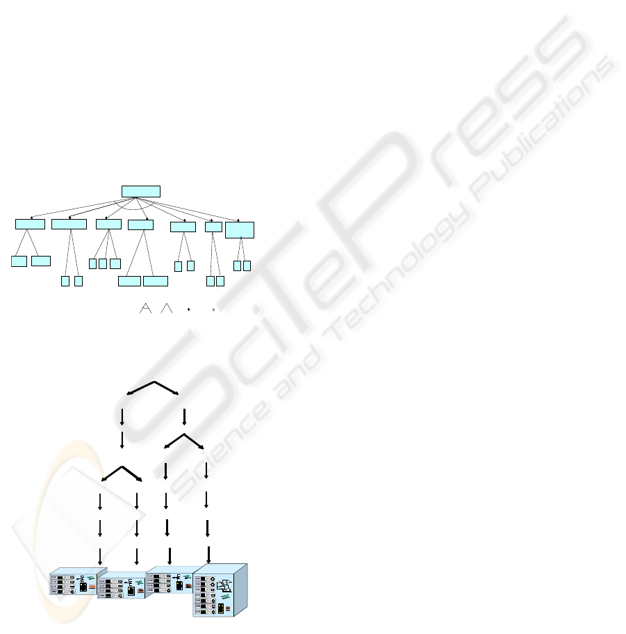
The features of the first variability type are

present in the Feature Model (FM) of our SPL

(Figure 2). These features are represented as

variability points in a DT. This DT allows the access

to the assets necessary to build base architectures

(i.e. the architectural elements, their feature insertion

processes, the base architectural model

configuration, the feature insertion main process, the

Application Domain Conceptual Model (ADCM),

and the Reusable Asset Specification (RAS)

(http://www.omg.org/technology/documents/formal/

ras.htm) model of assets. These assets are the leaves

of the DT (Figure 3). The FM and the DT act as

variability mechanisms that manage the variability at

the artefact level.

DIAGNOSIS

Property Levels

Reasoning

Hypothesis

same

change

1 2

deductive differential

Use Cases

Actors

1 2

Use Cases

by Actor

1 2

NOMENCLATURE:

and

(select 1)

mandatory

optional

4 14

Entity Views

Figure 2: Diagnostic Feature Model.

Reasoning

Property Levels

Use Cases

Actors

Hypotheses

Entity Views

same

change

deductive

differential

1-2

Use Cases by Actor

BOX 1

BOX 2

BOX 3

BOX 4

Figure 3: Diagnostic Decision Tree.

We have detected seven types of features (or

variability points) that are present in the FM and the

DT:

• entity views: an entity can be characterized by

the same properties (the same view), or have

different properties (different views) during the

diagnostic process.

• property levels: the properties of the entities can

have n different abstraction levels. The

deduction rules relate these properties between

levels.

• number of hypotheses: the goal of the

diagnostic process is a single hypothesis. There

can be one or several candidate hypotheses,

which must all be validated in order to obtain

the unique and correct hypothesis.

• reasoning types: reasoning shows the way in

which the rules are applied by the inference

motor in order to infer a final diagnosis. The

reasoning types can be: deductive reasoning

(driven by data), inductive reasoning (driven by

goals), and differential reasoning (establishing

the difference between two or more diagnostic

possibilities).

• number of use cases: a use case indicates the

division of the system based on its functionality;

i.e., the different operations of the systems and

how the system interacts with the environment

(final users).

• number of actors: represents the number of final

users of the system.

• use cases per actor: each final user can access

different use cases.

An example of these features applied to our

educational program diagnosis is: the entity views

are the same during the diagnostic process, there are

two property levels, one hypothesis, deductive

reasoning, one use case, one actor, and one use case

per actor. With this information, the assets that will

form the base architecture of this case study are

selected (Figure 3).

The variability shown in the use cases, actors,

and use cases per actor is reflected in the

construction of the assets of the architectural

element skeletons and in the base architecture in the

following way:

• there is one connector that joins all the

architectural component assets for each use

case,

• the number of ports of the Inference Process

component is the same as the number of use

cases,

• the number of ports of the Knowledge Base is

the number of use cases,

• the number of User Interfaces is the number of

actors of the use cases,

VARIABILITY MANAGEMENT IN SOFTWARE PRODUCT LINES FOR DECISION SUPPORT SYSTEMS

CONSTRUCTION

• the number of ports of the User Interface is the

number of use cases that can be accessed by an

actor.

The domain variability management could be

viewed as a transformation taking as input the

Domain Conceptual Model (DCM) and the Decision

Tree Model, and producing as output the

corresponding Base Architecture Model (we call it

T1).

The structure of the architectural elements

involves features on three variability points in the

DT. These features are used to select assets that let

to configure the base architectures.

The behaviour of the architectural elements

involves the features of four variability points in the

DT: entity views, property levels, number of

hypotheses, and reasoning types. These features are

related to the services, the protocols and the

played_roles of the aspects from the PRISMA

architectural elements (the information of state,

process, and roles, respectively).

To optimize the feature insertion process, instead

of repeating this information in each PRISMA type,

we have placed it in the skeletons of the Baseline.

4 VARIABILITY IN THE

APPLICATION DOMAIN: V2

The second type of variability involves the SPL of

the application in a specific field. This variability

allows to the base architectures to be enriched or

decorated with the application domain features.

In the process of the application variability

management, the variations of the specific

requirements of the application domain should be

selected. This selection is made by means of an

ADCM. The features are inserted (by means of

QVT-Transformations (http://www.omg.org/

docs/formal/05-07-01.pdf) in the base skeletons in

order to generate the types of the PRISMA software

artifacts. These PRISMA architectural elements will

be used to configure the PRISMA architectural

model of the application. That model is

automatically compiled into code (C#) using the

PRISMA Model Compiler (Cabedo et al., 2005), and

it is executable over the PRISMA NET Middleware

(Costa et al., 2005).

The features that are used to fill the skeletons to

obtain PRISMA types that make up the PRISMA

base architectures of our SPL are:

• name and type of the entity properties, that will

be diagnosed,

• name and type of the hypotheses,

• the rules that relate the entity properties.

In the following, we present an example of these

features (F) in our educational program diagnosis:

• Features of the properties of level 0 (FP.0) =

{student_population, graduation_rate,

graduation_time, graduate_quality,

control_school, critical_mass,

academic_training, scientific_productivity,

groups_lines_research, general_design,

pupil_control, research_experience_students,

number_courses, scheduled_duration, library,

computer_equipment, laboratories,

building&facilities, general_services }

• Features of the properties of level 1 (FP.1) =

{student_body, faculty, curriculum,

infrastructure&services }

• Features of the hypotheses (FH) =

developmental_stage

• Features of the rules of level 1 (FR.1) =

{student_population=”good” and

graduation_rate=”good” and

graduation_time=”good” and

graduate_quality=”good” and

control_school=”good” } student_body

=”good”

• Features of the rules of level 2 (FP.2) =

{student_body =” good” and faculty =” good”

and curriculum =” good” and

infrastructure&services=” good” }

developmental_stage = “consolidated”

The features considered as constants represent the

base models (in our case, the skeletons). For

example, S-IP-EPD, which means the “S-IP-EPD

program”. It is a constant feature. S-IP-EPD is the

nomenclature used for Inference Process Skeleton of

the Educational Program Diagnosis.

The skeletons selected will be filled or decorated

with the features of the application domain in order

to create the respective types. These types will

include the features as functions, which are

refinements of the base models. These models are

extensions of the base model, which is taken as

input. For example, F ● S-IP-EPD, wich means:

“insert the F feature into the S-IP-EPD model”,

where ● is the application of the F function. The

successive decoration process with features will be

represented as:

S-IP-EPD

= FP.0 ● S-IP-EPD

FP.0 ● (E-MI- DPE

)

S-IP-EPD

= FP.1 ● S-IP-EPD

FP.1 ● (E-MI- DPE

)

S-IP-EPD

= FH ●·S-IP-EPD

FH ● (E-MI- DPE

)

ICEIS 2008 - International Conference on Enterprise Information Systems

S-IP-EPD

= FR.1 ● S-IP-EPD

FR.1 ● (E-MI- DPE

)

S-IP-EPD

= FR.2 ● S-IP-EPD

FR.2 ● (E-MI- DPE

)

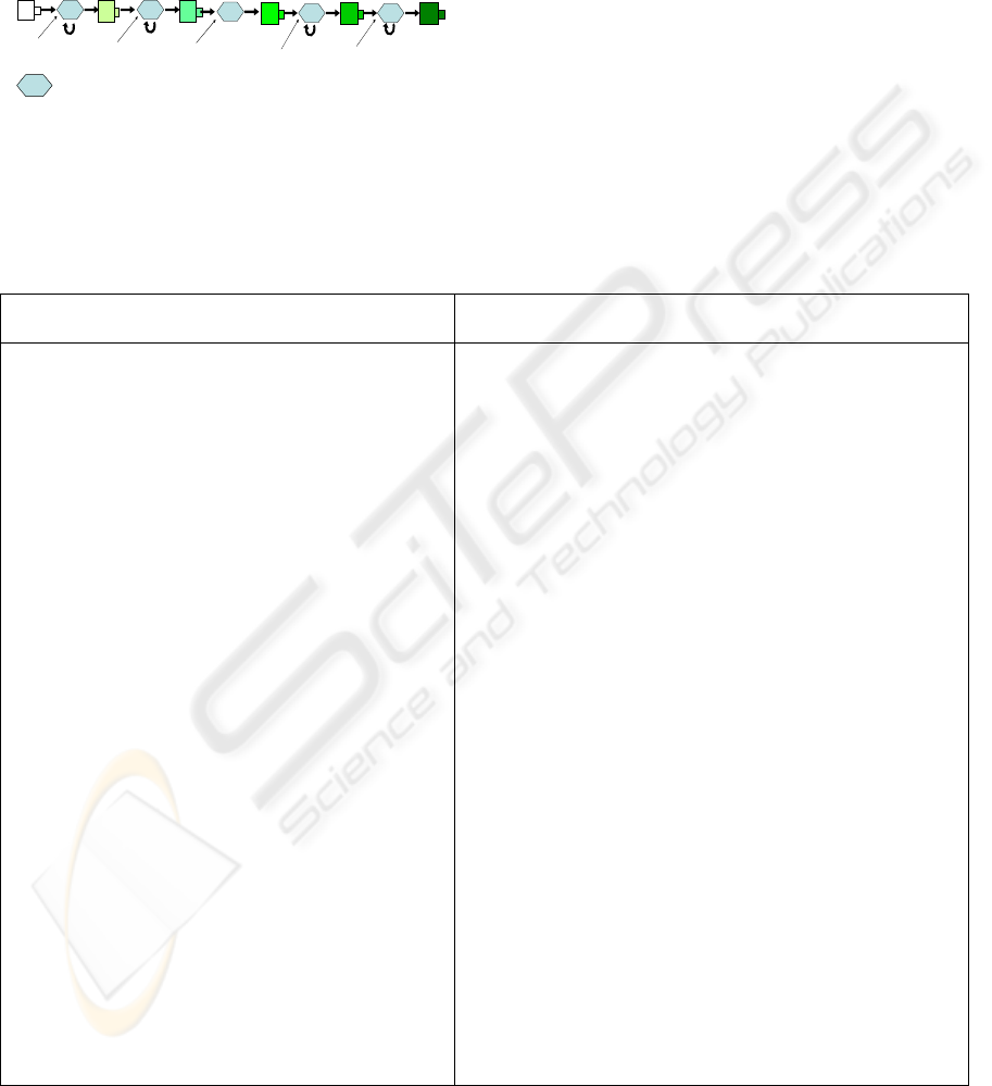
Figure 4 represents a visual metaphor of the feature

insertion process in a skeleton selected from the

Baseline (S-IP-EPD0) to create its PRISMA type.

= The j th transformation (feature insertion)

FP.0

FP.1

FP.0

FP.0,

FP.1

S-IP-EPD

FR.1

FR.2

FP.0, FP.1,

FH, FR.1

FP.0, FP.1,

S-IP-EPD

FP.0, FP.1,

FH, FR.1,

FR.2

Figure 4: Feature insertion process in a skeleton to create

its PRISMA type.

It is important to state that a Skeleton-Base

Architecture can be instantiated to one or more

PRISMA-Base Architecture types (i.e. several

products of our SPL), when the decorating features

are different. In two case studies performed by the

authors (the diagnosis of the developmental_stage of

educational programs, and the diagnosis of TV video

quality), they shared the same skeleton, but each one

of them has different PRISMA types. This was due

to the fact that different properties of the application

domain were inserted in each case.

As an example of this, we present in Table 1 the

functional aspect skeleton of the Knowledge Base

and the PRISMA type. Both the skeleton and the

type are specified in PRISMA-ADL (Architecture

Description Language).

Table 1: PRISMA-ADL of the Functional Aspect of the Knowledge Base (The different section holes are depicted in bold

type.

Functional aspect of the Knowledge Base

of a skeleton

Functional aspect of the Knowledge Base of a

PRISMA type

Functional Aspect FBaseEPD using

IDomainDPEDT

Attributes

Variables

<FP.0>

Derived

<FP.1>

<FH>

......

Derivations

<FR.1>

<FR.2>

........

Services

......

Played_Roles

........

Protocols

......

End_Functional Aspect FBaseEPD

Functional Aspect FBaseEPD using IDomainDPEDT

Attributes

Variables

laboratories:string,

library:string,

critical_mass:string,

scientific_productivity:string;

Derived

infrastructure&services:string,

faculty:string

developmental_stage:string;

......

Derivations

{laboratories=”good” and library=“good”}

infrastructure&services:=“good”

{critical_mass=”good” and

scientific_productivity =“good”} faculty:=

“good”

{infrastructure&services=“good” and faculty=

“good”} developmental_stage:=“consolidated”;

......

Services

......

Played_Roles

........

Protocols

......

End_Functional Aspect FBaseEPD

VARIABILITY MANAGEMENT IN SOFTWARE PRODUCT LINES FOR DECISION SUPPORT SYSTEMS

CONSTRUCTION

5 DESIGNING DECISION

SOFTWARE

ARCHITECTURES: PRODUCT

ENGINEERING PHASE

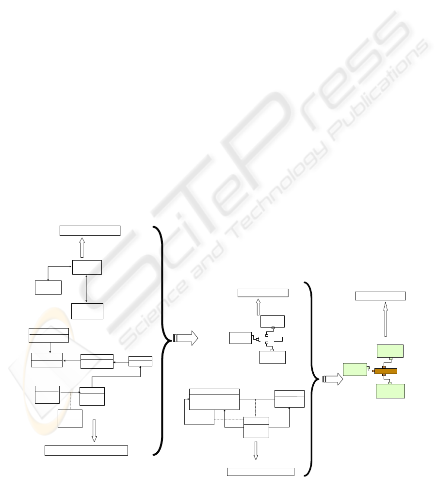
Figure 5 shows the transformations involved in the

design of the decision software architectures. This

figure illustrates how the two transformations

performed at the model level are applied in the

transformation process. Transformations T1 and

T2 are executed at the model level (M1 in OMG-

MOF (http://www.omg/org/mof) shown in Figure

5, they are defined as relations in QVT-Relational

at the metamodel level (M2 in OMG-MOF).

In transformation T1, the Component-

Connector (C-C) Skeleton model (c) is obtained

from the DSS modular model (a) and the DCM (b).

In transformation T2, the PRISMA architecture

model (e) is obtained from the Skeleton C-C model

generated in T1 (c) and the ADCM (d).

The relations R1 and R2 that specify the

corresponding transformations T1 and T2 are:

R1 ⊆ MM MODULAR VIEW X MMV1 →

def MM C-C SKELETON ;

R2 ⊆ MM C-C SKELETON X MMV2 →

def MM PRISMA VIEW ;

Where MMV1 and MMV2 are the metamodels

(MM) of the DCM and the ADCM. We use the

UML metamodel

(http://www.omg.org/docs/formal/05-07-04.pdf)

for both.

The relations R1 and R2 have been specified

using QVT-Relational. One of them is (R1

relations):

MODULAR VIEW → C-C VIEW

In BOM, the stakeholders only introduce the

variability data by means of the Conceptual

Models: In the fisrt step, the stakeholders introduce

the variability of the domain by means of the DCM

capturing the domain variability V1. T1 will obtain

a base architecture “ad hoc” to the case study using

the Generic Architecture Modular View. In the

second step, the stakeholders introduce the

variability of the application domain by means of

the ADCM capturing the application variability

V2. T2 will generate a PRISMA architecture

model as a product of our SPL (application

engineering), using the Skeleton C-C- model

generated in the first step. The two conceptual

models conform to their respective metamodels

(MM): the UML metamodel.

Modular Meta-model

UML-Class Meta-model: MMV

conforms_to

(a)

(b)

INFERENCE

MOTOR

KNOWLEDGE

BASE

USER

INTERFACE

Reasoning

Type: {deductive,

diferential,}

Use Cases

Number : nat

Actor

Number : nat

Use Cases

by Actor

Number : nat

Hypothesis

Number: nat

Property

Levels: nat

is_require

is_result

1..* 1

1..*

to_obtain

1..*

to_related

Entity View

Views: {same, change}

has

1..*

C-C View Meta-model

UML-Class Meta-model: MMV

conforms_to

(c)

(e)

(d)

C-C View Meta-model

INFERENCE

MOTOR

KNOWLEDGE

BASE

USER

INTERFACE

CONNECTOR

INFERENCE

MOTOR

KNOWLEDGE

BASE

USER

INTERFACE

CONNECTOR

Property

Name: string

Type: {string, nat, real, bool}

Level: nat

1..*

Property

Level n

Property

level n+1

Hypothesis

Name: string

Type: string

Rule

Clause: string

Level: nat

inferred

11..*

Figure 5: The transformation of models in BOM.

ICEIS 2008 - International Conference on Enterprise Information Systems

5.1 Specification of the Relations

between the Software Views

The relations between the software views are

specified by means of a MOF diagram, and the code

for these relations is written in the QVT-relational.

Code and diagrams are shown in (Limón et al.,

2007). In order to gain clarity the prefix “skeleton”

will be omitted from now, i.e “skeleton component”

will be written as “component”, and “skeleton

connector” will be written as “connector”. The

relations between the software views are the

following:

i) Relation moduleToComponent. This relation

maps each module with a component. Relation

moduleToComponent has two types of relations: the

checkonly type and the enforce type. The object of

the Module domain is of the checkonly type. In

contrast, the object of the Component domain is of

the enforce type. This creates an object of the

Component class that is related to the Module class.

The where clause indicates a call to the

functionToService relation, which relates an object

of the Module class with an object of the Component

class.

ii) Relation functionToService. This relation

implies that a function of the module metamodel

will generate a service of the Component class.

When this occurs, the type of the Function will

generate a port. In the where clause, the name of the

port is obtained by calling the function typePort.

When the relation is executed, the classes that are in

the source metamodel can only be verified and the

classes that are in the target meta-model will be

created (only the ServiceToPort class).

iii) Relation rUseModToConnector. The ‘uses’

relation is transformed from the modular meta-class

to a link between a connector and two components

in the C-C meta-class. The creation of objects for

this relation is from 1 to n because a relation of two

components is generated through a connector. In

(Limón et al., 2007) is shown part of the code to

illustrate how the relations are invoked in the

‘where’ clause to create the relations among module,

component, and functionToService.

iv) Relation rCompositionModToComp. The set

of modules will also generate a set of components.

However, in this case when a component is created

(container) a subordinate is created inside it.

6 CONCLUSIONS

The development of DSS is complex because there

is variability in the architectural elements that

conforms them as well as variability in their final

architecture. This situation produces several base

architectures in our SPL, sharing a unique generic

architecture.

Futhermore, the complexity problem of these

kind of systems is not solved by means of a unique

Feature Model and the insertion of its features. Since

the variability management is the essence of SPL,

we have taken a new approach. This approach

manages the variability in two stages, wich

correspond to the development of two SPL:

i) the base architectures SPL that shares a generic

architecture, and

ii) the application SPL in a specific domain, that

shares a base architecture.

In this context, we describe how the variability is

managed in our SPL by means of our BOM

framework. BOM automatically generates DSS in a

specific domain using SPL.

BOM captures the data that characterize the

domain variability and the application variability in

conceptual models. DT and FOM exploit this data in

the domain engineering and product engineering

phases in order to obtain a specific application by

means of Model Transformation techniques. In

BOM, the variability appears in the construction of

the DCM (which is represented as a DT showing the

different variation points). The base assets are

selected by the DT to configure a base architecture.

These assets are enriched by the specific application

features (given in the ADCM) by a process that

results in PRISMA types (a product of our LPS).

In the domain engineering phase, the user

constructs the different assets and stores them in the

Baseline. This Baseline is used in the application

engineering phase by a production plan in order to

obtain the final product. The production plan is one

of the assets stored in the Baseline.

We can conclude that the main characteristics of

BOM are the following:

i) Variability is managed at the model level

rather than at the program level.

ii) Systems variability is modeled using

conceptual models independently of their functional

models. The DSLs for expressing the variability are

suited for the domain, instead of adding tangled

variability annotations directly to the functional

models (UML, ADLs) as other approaches have

VARIABILITY MANAGEMENT IN SOFTWARE PRODUCT LINES FOR DECISION SUPPORT SYSTEMS

CONSTRUCTION

proposed (AMPLE project: http://www.ample-

project.net).

iii) Variability is operated by two orthogonal

types: one provided by the features of the domain

(e.g. diagnosis), and another one provided by the

features of the application domain.

iv) Various technological spaces are integrated to

cope with the complexity of the problem.They are

the current trends in Software Engineering.

v) BOM implements a generic approach to SPL

developement, that can be applied to different

domains, application domains and systems. In this

paper, the BOM framework is applied to the

diagnostic domain. Other domains will be

considered in the near future, e.g. interpretation, and

prediction.

A prototype of the BOM framework: ProtoBOM has

been implemented and will be used in real case

studies. In the future, we will use benchmarks in

order to compare BOM results with other

approaches.

ACKNOWLEDGEMENTS

This work has been funded under the Models,

Environments, Transformations, and Applications:

META project TIN20006-15175-605-01.

REFERENCES

Bachman F., Goedicke M., Leite J., Nord R., Pohl K.,

Ramesh B., and Vilbig A, 2003. “A meta-model for

representing variability in product family

development”, The 5th International Workshop on

Product Family Engineering, pp. 66-80.

Batory D., Benavides D., and Ruiz-Cortés A., 2006.

Automated Analyses of Feature Models: Challenges

Ahead. ACM on Software Product Lines.

Cabedo R., Pérez J., Carsí J.A. y Ramos I., 2005.

“Modelado y Generación de Arquitecturas PRISMA

con DSL Tools”, IV Workshop DYNAMICA, Murcia,

España. (in spanish)

Clements P. and Northrop L.M., 2002. Software Product

Lines: Practices and Patterns. SEI Series in Software

Engineering, Addison Wesley.

Costa C., Pérez J., Ali N., Carsí J.A. y Ramos I., 2005.

“PRISMANET: Middleware: Soporte a la Evolución

Dinámica de Arquitecturas Software Orientadas a

Aspectos”, X Jornadas de Ingeniería del Software y

Bases de Datos, Granada, España, pp. 27-34. (in

spanish)

González-Baixauli B. y Laguna M. A., 2005. “MDA e

Ingeniería de Requisitos para Líneas de Producto”,

Taller sobre Desarrollo Dirigido por Modelos. MDA y

Aplicaciones, Granada, España. (in spanish)

Limón Cordero R., Cabello Espinosa M.E., and Ramos

Salavert I., 2007. “Establish Relations among

Software Architecture Views through MDA for SPL”.

In Proceedings of the 14th International Congress on

Computer Science Research, CIICC'07, Veracruz,

México, ISBN 13 978-970-95771-0-5, pp. 175-187.

Pérez J., 2006. PRISMA: Aspect-Oriented Software

Architectures. PhD. Thesis of Philosophy in Computer

Science, Polytechnic University of Valencia, Spain.

Santos A.L., Koskimies K., and Lopes A., 2005. “Using

Model-Driven Architecture for Variability

Management in Software Product Lines”, Ph Thesis

Propasa, Facultade de Ciencias de la Universidade de

Lisboa, Portugal.

Trujillo S., 2007. Feature Oriented Model Driven Product

Lines. PhD. Thesis, The University of the Basque

Country, San Sebastian, Spain.

Turban, E., and Aronson, J.E., 2001. Decision Support

Systems and Intelligent Systems, Prentice Hall, ISBN:

0-13-089465-6, 865 pages.

ICEIS 2008 - International Conference on Enterprise Information Systems