Learning and Evolution in Artificial Neural Networks:

A Comparison Study

Eva Volna

University of Ostrava, 30

dubna st. 22, 701 03 Ostrava, Czech Republic

Abstract. This paper aims at learning and evolution in artificial neural

networks. Here is presented a system evolving populations of neural nets that

are fully connected multilayer feedforward networks with fixed architecture

solving given tasks. The system is compared with gradient descent weight

training (like backpropagation) and with hybrid neural network adaptation. All

neural networks have the same architecture and solve the same problems to be

able to be compared mutually. In order to test the efficiency of described

algorithms, we applied them to the Fisher's Iris data set [1] that is the bench

test database from the area of machine learning.

1 Learning in Artificial Neural Networks

Learning in artificial neural networks is typically accomplished using examples. This

is also called training in artificial neural networks because the learning is achieved by

adjusting the connection weights in artificial neural networks iteratively so that

trained (or learned) artificial neural networks can perform certain tasks. The essence

of a learning algorithm is the learning rule, i.e. a weight-updating rule, which

determines how connection weights are changed. Examples of popular learning rules

include the delta rule, the Hebbian rule, the anti-Hebbian rule, and the competitive

learning rule, etc. More detailed discussion of artificial neural networks can be found

in [2]. Learning in artificial neural networks can roughly be divided into supervised,

unsupervised, and reinforcement learning. Without commonness, we are going to

target multilayer feedforward neural networks that are adapted with backpropagation

algorithm.

Supervised learning is based on direct comparison between the actual output of an

artificial neural network and the desired correct output, also known as the target

output. It is often formulated as the minimization of an error function such as the total

mean square error between the actual output and the desired output summed over all

available data. A gradient descent-based optimization algorithm such as

backpropagation [2] can then be used to adjust connection weights in the artificial

neural network iteratively in order to minimize the error. There have been some

successful applications of backpropagation in various areas [3]–[5], but

backpropagation has drawbacks due to its use of gradient descent. It often gets

trapped in a local minimum of the error function and is incapable of finding a global

minimum if the error function is multimodal and/or nondifferentiable.

Volna E. (2008).

Learning and Evolution in Artiﬁcial Neural Networks: A Comparison Study.

In Proceedings of the 4th International Workshop on Artiﬁcial Neural Networks and Intelligent Information Processing, pages 10-17

DOI: 10.5220/0001506900100017

 SciTePress

2 NeuroEvolutionary Learning in Artificial Neural Networks

Evolutionary algorithms refer to a class of population-based stochastic search

algorithms that are developed from ideas and principles of natural evolution. They

include evolution strategies, evolutionary programming, genetic algorithms etc. [6].

One important feature of all these algorithms is their population based search strategy.

Individuals in a population compete and exchange information with each other in

order to perform certain tasks. Evolutionary algorithms are particularly useful for

dealing with large complex problems, which generate many local optima. They are

less likely to be trapped in local minima than traditional gradient-based search

algorithms. They do not depend on gradient information and thus are quite suitable

for problems where such information is unavailable or very costly to obtain or

estimate. They can even deal with problems where no explicit and/or exact objective

function is available. These features make them much more robust than many other

search algorithms. There is a good introduction to various evolutionary algorithms for

optimization in [6].

Evolution has been introduced into artificial neural networks at roughly three

different levels [7]: connection weights; architectures; and learning rules. The

evolution of connection weights introduces an adaptive and global approach to

training, especially in the reinforcement learning and recurrent network-learning

paradigm where gradient-based training algorithms often experience great difficulties.

The evolution of architectures enables artificial neural networks to adapt their

topologies to different tasks without human intervention and thus provides an

approach to automatic artificial neural network design as both connection weights and

structures can be evolved. The evolution of learning rules can be regarded as a

process of learning to learn in artificial neural networks where the adaptation of

learning rules is achieved through evolution. It can also be regarded as an adaptive

process of automatic discovery of novel learning rules.

The evolutionary approach to weight training in artificial neural networks consists

of two major phases. The first phase is to decide the representation of connection

weights, i.e., whether in the form of binary strings or real strings. The second one is

the evolutionary process simulated by an evolutionary algorithm, in which search

operators such as crossover and mutation have to be decided in conjunction with the

representation scheme. Different representations and search operators can lead to

quite different training performance. In a binary representation scheme, each

connection weight is represented by a number of bits with certain length. An artificial

neural network is encoded by concatenation of all the connection weights of the

network in the chromosome. The advantages of the binary representation lie in its

simplicity and generality. It is straightforward to apply classical crossover (such as

one-point or uniform crossover) and mutation to binary strings [6]. Real numbers

have been proposed to represent connection weights directly, i.e. one real number per

connection weight [6]. As connection weights are represented by real numbers, each

individual in an evolving population is then a real vector. Traditional binary crossover

and mutation can no longer be used directly. Special search operators have to be

designed. Montana and Davis [8] defined a large number of tailored genetic operators,

which incorporated many heuristics about training artificial neural networks. The idea

was to retain useful feature detectors formed around hidden nodes during evolution.

One of the problems faced by evolutionary training of artificial neural networks is

the permutation problem [7] also known as the competing convention problem. It is

caused by the many-to-one mapping from the representation (genotype) to the actual

artificial neural network (phenotype) since two artificial neural networks that order

their hidden nodes differently in their chromosomes will still be equivalent

functionally. In general, any permutation of the hidden nodes will produce

functionally equivalent artificial neural networks with different chromosome

representations. The permutation problem makes crossover operator very inefficient

and ineffective in producing good offspring. The role of crossover has been

controversial in neuroevolution as well as among the evolutionary computation

community in general. However, there have been successful applications using

crossover operations to evolve neural networks [9]. Compared with the mutation only

system, the performance of the system using crossover operations is in general better

and that it also helps to compress the overall size of search space faster.

3 Comparison between Evolutionary Training and

Gradient-based Training

The evolutionary training approach is attractive because it can handle the global

search problem better in a vast, complex, multimodal, and nondifferentiable surface.

It does not depend on gradient information of the error (or fitness) function and thus is

particularly appealing when this information is unavailable or very costly to obtain or

estimate. For example, the same evolutionary algorithms can be used to train many

different networks: recurrent artificial neural networks [10], higher order artificial

neural networks [11], and fuzzy artificial neural networks [12]. The general

applicability of the evolutionary approach saves a lot of human efforts in developing

different training algorithms for different types of artificial neural networks. The

evolutionary approach also makes it easier to generate artificial neural networks with

some special characteristics. For example, the artificial neural networks complexity

can be decreased and its generalization increased by including a complexity

(regularization) term in the fitness function. Unlike the case in gradient-based

training, this term does not need to be differentiable or even continuous. Weight

sharing and weight decay can also be incorporated into the fitness function easily.

However, evolutionary algorithms are generally much less sensitive to initial

conditions of training. They always search for a globally optimal solution, while a

gradient descent algorithm can only find a local optimum in a neighbourhood of the

initial solution.

4 Hybrid Training

Most evolutionary algorithms are rather inefficient in fine-tuned local search although

they are good at global search. This is especially true for genetic algorithms. The

efficiency of evolutionary training can be improved significantly by incorporating

a local search procedure into the evolution, i.e. combining evolutionary algorithm’s

global search ability with local search’s ability to fine tune. Evolutionary algorithms

can be used to locate a good region in the space and then a local search procedure is

used to find a near-optimal solution in this region. The local search algorithm could

be backpropagation [2] or other random search algorithms. Hybrid training has been

used successfully in many application areas: Lee [13] and many others used genetic

algorithms to search for a near-optimal set of initial connection weights and then used

backpropagation to perform local search from these initial weights. Their results

showed that the hybrid algorithm approach was more efficient than either the genetic

algorithm or backpropagation algorithm used alone. If we consider that

backpropagation often has to run several times in practice in order to find good

connection weights due to its sensitivity to initial conditions, the hybrid training

algorithm will be quite competitive. Similar work on the evolution of initial weights

has also been done on competitive learning neural networks [14] and Kohonen

networks [15].

It is interesting to consider finding good initial weights as locating a good region in

the weight space. Defining that basin of attraction of a local minimum as being

composed of all the points, sets of weights in this case, which can converge to the

local minimum through a local search algorithm, then a global minimum can easily be

found by the local search algorithm if an evolutionary algorithm can locate a point,

i.e. a set of initial weights, in the basin of attraction of the global minimum. Fig. 1

illustrates a simple case where there is only one connection weight in the artificial

neural networks. If an evolutionary algorithm can find an initial weight such as w

, it

would be easy for a local search algorithm to arrive at the globally optimal weight w

even though w

itself is not as good as w

Fig. 1. An illustration of using an evolutionary algorithm to find good initial weights such that

a local search algorithm can find the globally optimal weights easily. w

in this figure is an

optimal initial weight because it can lead to the global optimum w

using a local search

algorithm.

5 Experiments

In order to test the efficiency of described algorithms, we applied it to the Iris flower

data set or Fisher's Iris data set is a multivariate data set introduced by Sir Ronald

Aylmer Fisher as an example of discriminated analysis [1]. It is sometimes called

Anderson's Iris data set because Edgar Anderson collected the data to quantify the

geographic variation of Iris flowers in the Gaspe Peninsula. The dataset consists of 50

samples from each of three species of Iris flowers (Iris setosa, Iris virginica and Iris

versicolor). Four features were measured from each sample, they are the length and

the width of sepal and petal. Based on the combination of the four features, Fisher

developed a linear discriminated model to determine which species they are (see

Table 1). There are three-layer feedforward neural networks with architecture

is 4 - 4 - 3 (e.g. four units in the input layer, four units in the hidden layer, and three

units in the output layer) in all experimental works, because the Fisher's Iris data set

[1] is not linearly separable and therefore we cannot use neural network without

hidden units. All nets are fully connected. The input values of the training set from the

Table 1 are transformed into interval <0; 1> to be use backpropagation algorithms for

adaptation.

Weight Evolution in Artificial Neural Networks: the initial population contains

30 individuals (weight representations of three-layer neural networks). There are

connection weights represented by real numbers in each chromosome. We use the

genetic algorithm with the following parameters: probability of mutation is 0,01 and

probability of crossover is 0,5. Adaptation of each neural network starts with

randomly generated weight values in the initial population.

The Gradient Descent adaptation deals through backpropagation with the

following parameters: learning rate is 0.4, momentum is 0.

The Hybrid Training combines parameters from genetic algorithms and

backpropagation. It makes one backpropagation epoch with probability 0,5 in each

generation.

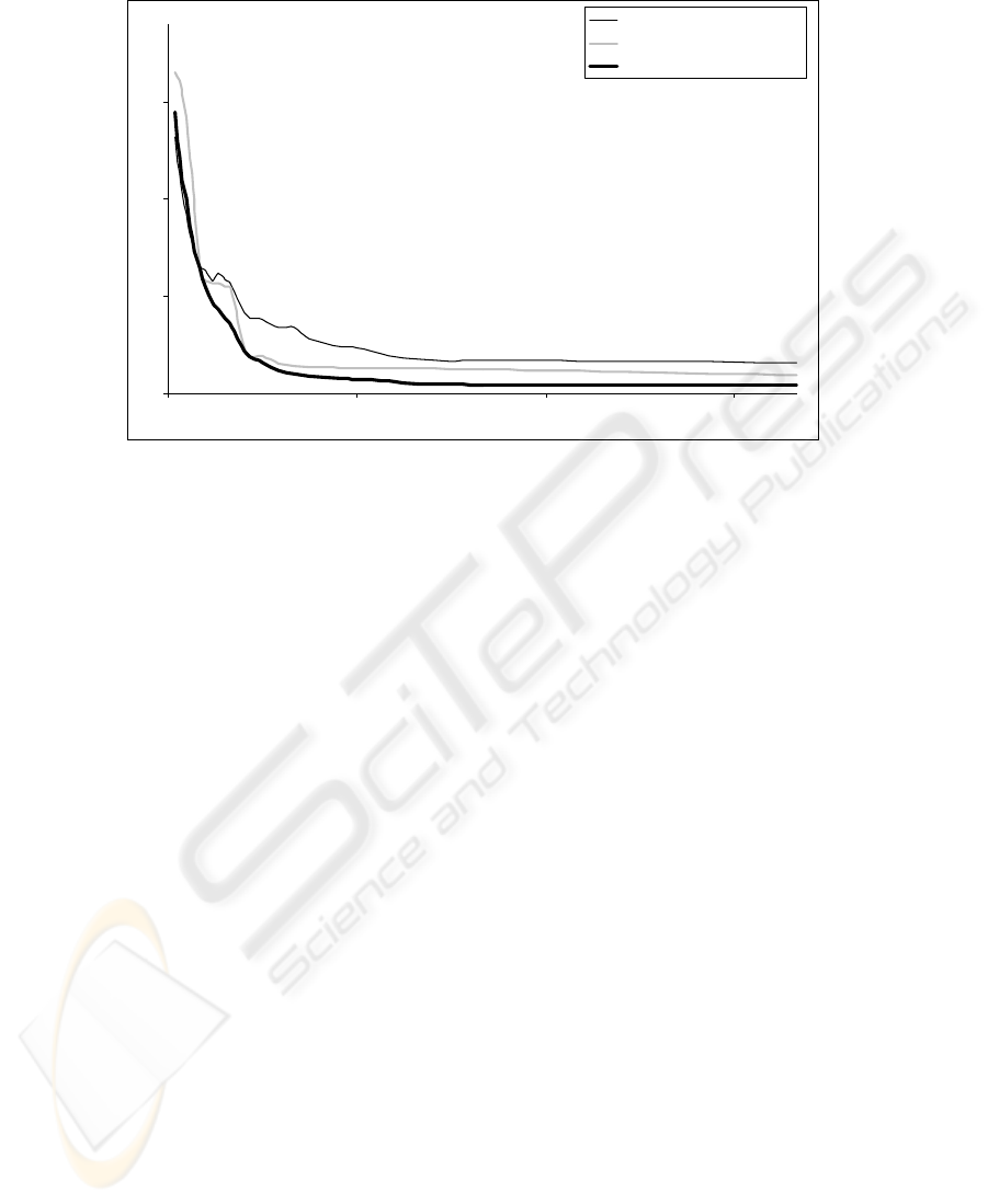
6 Conclusions

History of error functions is shown in the Figure 2. There are shown average values of

error functions in the given population. The “gradient descent adaptation” represents

an adaptation with the backpropagation. There are shown average values of error

functions, because the adaptation with backpropagation algorithm was applied 10

times for each calculation.

All networks solve Fisher's Iris data set [1] in our experiment. Now we can

compare results from all experiments, e.g. weight evolution, gradient descent

adaptation, and hybrid training. Other numerical simulations give very similar results.

If we can see from Figure 2, the hybrid training shows the best results from all of

them. In general, hybrid algorithms tend to perform better than others for a large

number of problems, because they combine evolutionary algorithm’s global search

ability with local search’s ability to fine tune

Table 1. The set of patterns (the Fisher's Iris Data training set), where Se means setosa,

Vi means virginica, and Ve means versicolor.

Sepal

Lengt

Sepal

Width

Petal

Length

Petal

Width

Spe-

cies

Sepal

Lengt

Sepal

Width

Petal

Length

Petal

Width

Spe-

cies

Sepal

Lengt

Sepal

Width

Petal

Length

Petal

Width

Spe-

cies

5,1 3,5 1,4 0,2

6,3 3,3 6 2,5

7 3,2 4,7 1,4

4,9 3 1,4 0,2

5,8 2,7 5,1 1,9

6,4 3,2 4,5 1,5

4,7 3,2 1,3 0,2

7,1 3 5,9 2,1

6,9 3,1 4,9 1,5

4,6 3,1 1,5 0,2

6,3 2,9 5,6 1,8

5,5 2,3 4 1,3

5 3,6 1,4 0,2

6,5 3 5,8 2,2

6,5 2,8 4,6 1,5

5,4 3,9 1,7 0,4

7,6 3 6,6 2,1

5,7 2,8 4,5 1,3

4,6 3,4 1,4 0,3

4,9 2,5 4,5 1,7

6,3 3,3 4,7 1,6

5 3,4 1,5 0,2

7,3 2,9 6,3 1,8

4,9 2,4 3,3 1

4,4 2,9 1,4 0,2

6,7 2,5 5,8 1,8

6,6 2,9 4,6 1,3

4,9 3,1 1,5 0,1

7,2 3,6 6,1 2,5

5,2 2,7 3,9 1,4

5,4 3,7 1,5 0,2

6,5 3,2 5,1 2

5 2 3,5 1

4,8 3,4 1,6 0,2

6,4 2,7 5,3 1,9

5,9 3 4,2 1,5

4,8 3 1,4 0,1

6,8 3 5,5 2,1

6 2,2 4 1

4,3 3 1,1 0,1

5,7 2,5 5 2

6,1 2,9 4,7 1,4

5,8 4 1,2 0,2

5,8 2,8 5,1 2,4

6,7 3,1 4,4 1,4

5,7 4,4 1,5 0,4

6,4 3,2 5,3 2,3

5,6 2,9 3,6 1,3

5,4 3,9 1,3 0,4

6,5 3 5,5 1,8

5,6 3 4,5 1,5

5,1 3,5 1,4 0,3

7,7 3,8 6,7 2,2

5,8 2,7 4,1 1

5,7 3,8 1,7 0,3

7,7 2,6 6,9 2,3

5,6 2,5 3,9 1,1

5,1 3,8 1,5 0,3

6 2,2 5 1,5

6,2 2,2 4,5 1,5

5,4 3,4 1,7 0,2

6,9 3,2 5,7 2,3

5,9 3,2 4,8 1,8

5,1 3,7 1,5 0,4

5,6 2,8 4,9 2

6,1 2,8 4 1,3

4,6 3,6 1 0,2

7,7 2,8 6,7 2

6,3 2,5 4,9 1,5

5,1 3,3 1,7 0,5

6,3 2,7 4,9 1,8

6,1 2,8 4,7 1,2

4,8 3,4 1,9 0,2

6,7 3,3 5,7 2,1

6,4 2,9 4,3 1,3

5 3 1,6 0,2

7,2 3,2 6 1,8

6,6 3 4,4 1,4

5 3,4 1,6 0,4

6,2 2,8 4,8 1,8

6,8 2,8 4,8 1,4

5,2 3,5 1,5 0,2

6,1 3 4,9 1,8

6,7 3 5 1,7

5,2 3,4 1,4 0,2

6,4 2,8 5,6 2,1

6 2,9 4,5 1,5

4,7 3,2 1,6 0,2

7,2 3 5,8 1,6

5,7 2,6 3,5 1

4,8 3,1 1,6 0,2

7,4 2,8 6,1 1,9

5,5 2,4 3,8 1,1

5,4 3,4 1,5 0,4

7,9 3,8 6,4 2

5,5 2,4 3,7 1

5,2 4,1 1,5 0,1

6,4 2,8 5,6 2,2

5,8 2,7 3,9 1,2

5,5 4,2 1,4 0,2

6,3 2,8 5,1 1,5

6 2,7 5,1 1,6

4,9 3,1 1,5 0,2

6,1 2,6 5,6 1,4

5,4 3 4,5 1,5

5 3,2 1,2 0,2

7,7 3 6,1 2,3

6 3,4 4,5 1,6

5,5 3,5 1,3 0,2

6,3 3,4 5,6 2,4

6,7 3,1 4,7 1,5

4,9 3,6 1,4 0,1

6,4 3,1 5,5 1,8

6,3 2,3 4,4 1,3

4,4 3 1,3 0,2

6 3 4,8 1,8

5,6 3 4,1 1,3

5,1 3,4 1,5 0,2

6,9 3,1 5,4 2,1

5,5 2,5 4 1,3

5 3,5 1,3 0,3

6,7 3,1 5,6 2,4

5,5 2,6 4,4 1,2

4,5 2,3 1,3 0,3

6,9 3,1 5,1 2,3

6,1 3 4,6 1,4

4,4 3,2 1,3 0,2

5,8 2,7 5,1 1,9

5,8 2,6 4 1,2

5 3,5 1,6 0,6

6,8 3,2 5,9 2,3

5 2,3 3,3 1

5,1 3,8 1,9 0,4

6,7 3,3 5,7 2,5

5,6 2,7 4,2 1,3

4,8 3 1,4 0,3

6,7 3 5,2 2,3

5,7 3 4,2 1,2

5,1 3,8 1,6 0,2

6,3 2,5 5 1,9

5,7 2,9 4,2 1,3

4,6 3,2 1,4 0,2

6,5 3 5,2 2

6,2 2,9 4,3 1,3

5,3 3,7 1,5 0,2

6,2 3,4 5,4 2,3

5,1 2,5 3 1,1

5 3,3 1,4 0,2

5,9 3 5,1 1,8

5,7 2,8 4,1 1,3

0 300 600 900

evolution

gradient descent adaptation

hybrid training

tim e

Error

Fig. 2. The error function history.

References

1. http://en.wikipedia.org/wiki/Iris_flower_data_set (from 16/1/2008)

2. Hertz, J., Krogh, A., and Palmer, R. Introduction to the Theory of Neural Computation.

Reading, MA: Addison-Wesley, 1991.

3. Lang, K. J. Waibel, A. H., and Hinton, G. E.“A time-delay neural network architecture for

isolated word recognition,” Neural Networks, vol. 3, no. 1, pp. 33–43, 1990.

4. Fels S. S. and Hinton, G. E. “Glove-talk: A neural network interface between a data-glove

and a speech synthesizer,” IEEE Trans. Neural Networks, vol. 4, pp. 2–8, Jan. 1993.

5. Knerr, S., Personnaz, L., and G. Dreyfus, “Handwritten digit recognition by neural

networks with single-layer training,” IEEE Trans, Neural Networks, vol. 3, pp. 962–968,

Nov. 1992, neural networks that uses genetic-algorithm techniques.”

6. Bäck, T., Hammel, U., and Schwefel, H.-P. “Evolutionary computation: Comments on the

history and current state”. IEEE Trans, Evolutionary Computation, vol. 1, pp. 3–17, Apr. 1997.

7. Yao, X. “Evolving artificial neural networks”, In Proceedings of the IEEE 89 (9) 1423-1447,

1999.

8. Montana, D., and Davis, L. “Training feedforward neural networks using genetic

algorithms.” In Proceedings 11th Int. Joint Conf. Artificial Intelligence, pp. 762–767San

Mateo, CA: Morgan Kaufmann, 1989.

9. Pujol, J. C. F. and Poli, R. Evolving the topology and the weights of neural networks using

a dual representation, Applied Intelligence, 8(1):73–84, 1998.

10. Angeline, P. J., Saunders, G, M., and Pollack, J. B. An evolutionary algorithm that

constructs recurrent neural networks, IEEE Transactions on Neural Networks, pages 54–65,

1994.

11. Janson D. J. and Frenzel, J. F. “Application of genetic algorithms to the training of higher

order neural networks,” J, Syst, Eng., vol. 2, pp. 272–276, 1992.

12. Lehotsky, M. Olej, V. and Chmurny, J. “Pattern recognition based on the fuzzy neural

networks and their learning by modified genetic algorithms,” Neural Network World, vol.

5, no. 1, pp. 91–97, 1995.

13. Lee, S.-W. “Off-line recognition of totally unconstrained handwritten numerals using

multilayer cluster neural network,” IEEE Trans. Pattern Anal. Machine Intell., vol. 18, pp.

648–652, June 1996.

14. Merelo, J. J. Paton, M. Canas, A., Prieto, A. and Moran, F. “Optimization of a competitive

learning neural network by genetic algorithms,” in Proc. Int. Workshop Artificial Neural

Networks (IWANN’93), Lecture Notes in Computer Science, vol. 686, Berlin, Germany:

Springer-Verlag, 1993, pp. 185–192.

15. Wang, D. D. and Xu, J. “Fault detection based on evolving LVQ neural networks,” in Proc.

1996 IEEE Int. Conf. Systems, Man and Cybernetics, vol. 1, pp. 255–260.