EFFICIENT PLANNING OF AUTONOMOUS ROBOTS USING
HIERARCHICAL DECOMPOSITION
Matthias Rungger, Olaf Stursberg
Institute of Automatic Control Engineering, Technische Universit¨at M¨unchen, 80333 Munich, Germany
Bernd Spanfelner, Christian Leuxner, Wassiou Sitou
Software and System Engineering, Technische Universit¨at M¨unchen, 80333 Munich, Germany
Keywords:
Hierarchical Planning, Autonomous Robots, Context Adaptation, Hybrid Models, Predictive Control.
Abstract:
This paper considers the behavior planning of robots deployed to act autonomously in highly dynamic envi-
ronments. For such environments and complex tasks, model-based planning requires relatively complex world
models to capture all relevant dependencies. The efficient generation of decisions, such that realtime require-
ments are met, has to be based on suitable means to handle complexity. This paper proposes a hierarchical
architecture to vertically decompose the decision space. The layers of the architecture comprise methods for
adaptation, action planning, and control, where each method operates on appropriately detailed models of the
robot and its environment. The approach is illustrated for the example of robotic motion planning.
1 INTRODUCTION
The spectrum of applications for future robots will
continuously grow, and an increasing percentage will
be employed in dynamic environments. Examples
are service robots which assist elderly or disabled
persons and rescue robots which operate in hostile
areas that are devastated by earthquakes or similar
incidents. A characteristic of such applications is
that an autonomous planning of actions must consider
changing environment conditions and include reliable
and immediate decisions on which available resources
should be employed to fulfill a momentary task. In
particular, if the environment includes dynamic ob-
jects with non-deterministic or partly unpredictable
behavior, the representation of the constraints for a
planning problem becomes complex and has a signif-
icant impact on the realtime-computability of action
plans. Another difficulty encountered in this case is
that environment models which are purely identified
based on data series measured over a short period of
time for a specific situation are merely suitable to re-
flect the behavior of the environment sufficiently well.
In order to cope with the issues of model complex-
ity and quality of prediction within action planning,
this paper proposes a planning architecture which
combines multi-layer decision making with the use of
a knowledge base for storing learned goal-attaining
action strategies. Of course, the idea of hierarchi-
cal planning architectures is not new in general, and
corresponding approaches can be found, e.g., in (Nau
et al., 1998), (Galindo et al., 2007), (Barto and Ma-
hadevan, 2003). However, the novel contribution of
this paper is that a three-tier scheme is suggested
which separates the planning task into steps of config-
uring the system structure, of planning a sequence of
actions, and refining these actions into locally optimal
control trajectories. The configuration step allocates
the set of resources (sensors, actuators, or algorithms
for planning and control) that seem most appropriate
to accomplish a given task. By employing reinforce-
ment learning, the action planning on a medium layer
produces a sequence of discrete actions that qualita-
tively accomplish the task. The third layer refines an
action plan by generating control trajectories which
correspond to the action plan and establish a quanti-
tative setting for the actuators over time. The overall
concept setting is explained in the following section.
262
Rungger M., Stursberg O., Spanfelner B., Leuxner C. and Sitou W. (2008).
EFFICIENT PLANNING OF AUTONOMOUS ROBOTS USING HIERARCHICAL DECOMPOSITION.
In Proceedings of the Fifth International Conference on Informatics in Control, Automation and Robotics - RA, pages 262-267
DOI: 10.5220/0001502202620267
Copyright
c
 SciTePress

2 HIERARCHICAL PLANNING
APPROACH
The proposed hierarchy vertically decomposes a com-
plex planning task for reduction of complexity wher-
ever possible, and consists of the layers shown in
Fig.1: The adaptation-layer perceives and evaluates
the current situation based on measured data and de-
cides on the configuration, i.e. the resources selected
to solve a current task. The planning layer consid-
ers the allocated resources and existing constraints for
calculating an action plan that accomplishes the task.
In the opposite direction, information about the ex-
istence of a feasible plan for the chosen configura-
tion is transmitted from the planning to the adaptation
layer. The control layer refines the action sequences
received from the planning layer by computing a con-
trol trajectory for each action. The control trajectory
is then passed to the corresponding actuators of the
system. If no feasible trajectory is found for an ac-
tion (or a part of the action sequence), this informa-
tion is passed by to the planning layer and triggers
replanning. Thus, the three layers continuously inter-
act during the online execution to compute a task ac-
complishing strategy. To enable this computation, the
system must have the capability to predict the behav-
ior of itself and its environmentup to a point of time in
which the task is accomplished or cannot be accom-
plished anymore. These predictions are obtained from
evaluating the models shown in Fig. 1 for a choice of
configurations, action sequences, and control strate-
gies.
The hierarchy implements a nested feedback loop
also in the following sense: as soon as a current sit-
uation changes (e.g. because either a task changes
or a relevant change of the environment is detected)
the previously generated configuration, action plan, or
control trajectory is re-evaluated and possibly modi-
fied. The reactivity to the behavior of the environ-
ment requires continuous update of the models based
on measurement signals from the sensors of the au-
tonomous system. On each layer, appropriate identi-
Models
Configurations
State transition
systems
Hybrid Automata
Adaptation Layer
Planning Layer
Control Layer
Knowledge
base
Figure 1: The hierarchical architecture.
fication techniques are included to reparametrize the
models to the momentarily perceived situation.
In summary, the main objective of the three-tier
architecture is (a) to decompose the decision making
into three qualitatively distinct categories, (b) to se-
lect components, algorithms, and behavior in a top-
down manner to reduce the search effort in the deci-
sion space, and to (c) include a knowledge-base by
which already ’experienced’ (or learned) behavior is
used as heuristics for efficiently deciding which strat-
egy is goal-attaining. For this scheme, the claim is
not to outperformsingle state-of-the-art algorithms on
a particular layer, but to provide an architecture for
proper integration of different algorithms to solve a
broad variety of complex planning tasks.
3 ADAPTATION LAYER
The term adaptation is here understood as the capa-
bility of an autonomous system to react to changing
tasks or varying aspects of the context in which the
system is embedded. The term ’context’ refers to the
state of the system environment, as e.g. the proximity
of obstacles to a moving robot (the ’system’). The
adaptation on the uppermost layer of the hierarchy
means here to deduce from the current context and
a task to be accomplished a suitable configuration,
which is a subset of available components, i.e. avail-
able hardware devices (e.g. actuators) or software
algorithms for action planning and control.
Components. On the adaptation layer, the system
and its environment are described in terms of com-
municating units called components. Formally, a
system is defined as a pair (C,CH) with C as a set
of components and CH as a set of channels. The
components communicate through directed channels,
which are defined by ch = C×C× Id with Id as a set
of unique names. A system is completely determined
by a network of components connected via channels,
and the components send messages along channels
and thereby express their behavior. Different ways
to describe such behavior exist, like e.g. process
algebras or relations on inputs and outputs like
FOCUS (Broy and Stoelen, 2001) or COLA (Haberl
et al., 2008). The behavior of a component is here
specified by a sequence of data msg ∈ MSG which
is received and sent over the ports I and O of the
component.
Adaptation Mechanism. To formalize the adapta-
tion of a component-based model, the notion of Mode
Switch Diagrams (MSD) is introduced. An MSD is
EFFICIENT PLANNING OF AUTONOMOUS ROBOTS USING HIERARCHICAL DECOMPOSITION
263

a tuple (M,map,δ,m
0
) defining a transition system
with a set of modes M, a transition function δ, a func-
tion map : m → C that relates modes to components,
and m
0
is the initial mode. The transitions are defined
by δ : M× P → M with predicates P depending on the
inputs i ∈ I of the components assigned to a mode.
The function δ encodes the transition of the MSD be-
tween two modes m
i
and m
i+1
, and it represents the
adaptation. An example of an adaptation is shown in
Fig. 2. An activated mode m
i+1
determines the com-
ponents of the system which are selected until a new
context change triggers another transition. The mode
constitute the frame for the action planning carried
out on the medium layer.
m
1
m
2
c
1
c
2
c
3
δ
1
I
I
O
O
Figure 2: Transition between two modes m
1
and m
2
of an
MSD example.
4 PLANNING LAYER
The planning layer comprises algorithms that search
for a sequence of actions which transfers the ini-
tial state of the system or environment into a desired
goal state. The specific algorithm to be used for a
given task, the available set of actions, and the rel-
evant model is determined by the mode information
received from the adaptation layer. The model used
on the planning layer is specified as a state transition
system Σ = (S,A, δ) consisting of a set of states S =
{s
1
,s
2
,... ,s
n
}, a set of actions A = {a
1
,a
2
,... ,a
m
},
and a transition function δ : S× A → 2
S
. The planning
task is mapped into a goal state s
G
(or a set of goal
states S
G
⊆ S, respectively) which has to be reached
from a current state s
0
∈ S. A plan is a sequence of
actions that evokes a state path ending in s
G
(or an
s ∈ S
G
).
The planning techniques on the medium layer fol-
low the principle of reinforcement learning. In order
to formulate the planning problem as optimization, an
utility function r : S× S → R is introduced, which de-
fines the reward of taking a transition of Σ. The goal
is encoded implicitly by assigning a high reward to a
state sequence via which a goal state is reached, and
by producing a negative reward for undesired behav-
ior of Σ. Reinforcement learning represents learning
from interaction, i.e. the system learns a strategy (as a
state-to-action mapping) based on the reward. At time
t, the system observes the state s ∈ S, and for a cur-
rent policy π = P(a|s) an action a ∈ A is chosen. The
system moves from state s to s
′
according to the tran-
sition function, and it receives the reward r. The goal
is to learn a policy π which maximizes the cumulative
discounted future reward. By introducing the action-
value function Q(s,a), a measure is available which
estimates the profit of taking an action a in state s.
The action-value function under policy π is given by
the Bellman equation:
Q
π
(s,a) = [R(s
′
|s,a) + γ
∑
a
′
π(s
′
,a
′
)Q
π
(s
′
,a
′
)],
where s
′
and a
′
denote state and action at the next time
instant. γ is the discount factor and is given by 0 <
γ < 1. R(s
′
|s,a) denotes the reward for taking action
a in state s, resulting in the new state s
′
. If the reward
function as well as the system dynamics are known,
the optimal policy
Q
∗
= max
π
Q
π
(s,a)
can be calculated explicitly, resulting in a system of
|S| · |A| equations. Since this is often computation-
ally intractable (in addiion to some dynamics may not
be known before-hand) approximations to the optimal
action-value function are used.
One possible algorithm to estimate Q
∗
(s,a) is
called SARSA (Takadama and Fujita, 2004), which
learns the current state-value function Q(s,a) by up-
dating the function with the observed reward, while
interacting with the environment:
Q(s,a) ← Q(s,a) + α[r + γQ
π
(s
′
,a
′
) − Q(s,a)],
where α is the learning rate. SARSA is a so called on-
policy RL algorithm, which updates the action-value
function while following a policy π. The policy is ε-
greedy, where the greedy action a
∗
= argmax
a
Q(s,a)
is selected most of the time. Once in a while, with
probability ε, an action is chosen randomly. SARSA
is used here as RL technique in order to reduce the
“risk” by avoiding negative rewards while paying
with a loss of optimality (Takadama and Fujita, 2004).
5 CONTROL LAYER
The control layer ensures the correct execution of the
action sequence derived on the planning layer. It es-
tablishes a connection of the discrete actions received
from the medium layer to the real world by apply-
ing continuous signals to the system’s actuators. The
combination of discrete actions with continuous dy-
namics motivates the use of hybrid automata (Hen-
zinger, 1996) to model the behavior on the control
layer. Hybrid automata (HA) do not only establish
ICINCO 2008 - International Conference on Informatics in Control, Automation and Robotics
264

an adequate interface to the higher layers, but also
provide the necessary expressivity required to model,
e.g. robot-object-interaction. For each component se-
lected by the adaptation layer, one hybrid automaton
is introduced, and the various automata can interact
via synchronization or shared variables.
Using a variant of HA with inputs according to
(Stursberg, 2006), a hybrid automaton modeling the
system is given by HA = (X,U,Z,inv, Θ,g, f), with
X as the continuous state space, U the input space,
Z the set of discrete locations, inv the assignment
of invariance sets for the continuous variables of
the discrete locations, and Θ the set of discrete
transitions. A mapping g : Θ → 2
z
associates a
guard set with each transition. The discrete-time
continuous dynamics f defining the system dynamics
is x(t
j+k
) = f(z(t
k
),x(t
k
),u(t
k
)). At any time t
k
, the
pair of continuous and discrete state forms the current
hybrid state s(t
k
) = (z(t
k
),x(t
k
)). Hybrid automata
for modeling relevant components of the environment
introduced without input sets U (since not directly
controllable).
Model Predictive Control. In order to generate con-
trol trajectories for the HA, the principle of model pre-
dictive control (MPC) is used (Morari et al., 1989).
Considering the control problem not only as a motion
planning problem like typically done in the robotic
domain, e.g. (LaValle, 2006), but as an MPC prob-
lem has the following advantages: (1) an optimal so-
lution for a given cost function and time horizon is
computed, (2) model-based predictions for the behav-
ior of the system and the environment lead to more
reliable and robust results, and (3) a set of differential
and dynamic constraints can be considered relatively
easy. The MPC scheme solves, at any discrete point
of time t
h
, an optimization problem over a finite pre-
diction horizon to obtain a sequence of optimal con-
trol inputs to the system. The optimization problem
considers the dynamics of the system and the follow-
ing additional constraints: a sequence of forbidden re-
gions φ
F,k
= {F
k
,F
k+1
, ·· · ,F
k+p
}, and a sequence of
goal regions φ
G,k
= {G
k
,G
k+1
, · ·· ,G
k+p
} are speci-
fied over the prediction horizon p·(t
k
−t
k−1
). Here, F
k
denotes a state region that the system must not enter,
and G
k
is the state set into which the system should
be driven. The constrained optimization problem can
be formulated as:
min
φ
u,k
J(φ
s,k
,φ
e,k
,φ
u,k
, p,φ
G,k
)
s.t. s(t
j
) /∈ F
j
∀ j ∈ {k, ...,k + p}
u
min
≤ u(t
j
) ≤ u
max
φ
s,k
∈ Φ
s
and φ
e,k
∈ Φ
e
where φ
s,k
and φ
e,k
are the predicted state trajectories
of the system and the environment, which must be
contained in the sets of feasible runs Φ
s
and Φ
e
. No
state s(t
j
) contained in φ
s,k
must be in a forbidden
region F(t
j
). u
min
and u
max
are the limitations for the
control inputs u(t
j
) and thus for the control trajectory
φ
u,k
. A possible solution technique for the above
optimization problem is the following sequential
one: (1) an optimizer selects a trajectory φ
u,k
, (2)
the models of system and environment are simulated
for this choice leading (possibly) to feasible φ
s,k
and φ
e,k
, (3) the cost function J is evaluated for
these trajectories, and (4) the results reveals if φ
u,k
should be further modified for improvement of the
costs or if the optimization has sufficiently converged.
Knowledge Base and Learning. In order to improve
the computational efficiency, the MPC scheme is en-
hanced by a knowledge-base, in which assignments
of action sequences to situations is stored. The ob-
jective of the learning unit with a knowledge base
is to reduce the computational effort by replacing
or efficiently initializing the optimization. The sit-
uations in the knowledge base are formulated as tu-
ple δ = (φ
s,k
,φ
e,k
,φ
G,k
,φ
F,k
,φ
u,k
,J), where s(t
k
) and
e(t
k
) again denote the current state of the system and
the environment, and φ
u,k
, φ
G,k
, and φ
F,k
are the se-
quences of control inputs, the goal, and forbidden
sets, respectively. For a given situation at the current
time t
k
, by using similarity comparison
1
, the learning
unit infers a proper control strategy φ
L
u,k
if it exists.
Otherwise, the optimization is carried out and the re-
sult is stored in the knowledge-base.
6 APPLICATION TO A KITCHEN
SCENARIO
The presented hierarchical architecture is applied to
a service robot in a kitchen scenario. The task of the
robot is to lay a table (see Fig 3), i.e. the robot is
expected to drive back and forth between a table and
a kitchenette for positioning plates and cutlery on
the table. The scenario obviously formulates a very
challenging planning task, as the robot has to decide
which object to take, how to move to the desired place
at the table, and how to avoid collision with humans
moving in the same space – this is the motivation
for employing a decomposition-based planning
approach. To simplify the upcoming presentation, the
1
Similarity is here defined by small distances of the
quantities specifying a situation in the underlying hybrid
state space.
EFFICIENT PLANNING OF AUTONOMOUS ROBOTS USING HIERARCHICAL DECOMPOSITION
265

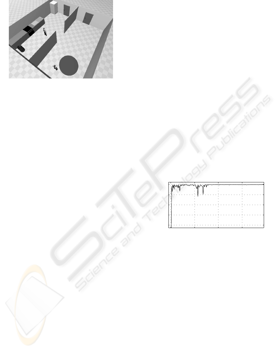
Figure 3: Setting of the kitchen scenario.
further discussion is here restricted here to the part of
robot motion planning only.
Adaptation. On the uppermost layer, the set of
components C comprises the relevant physical com-
ponents of the setting and the choice of algorithms
being available on the planning and control lay-
ers. Thus, the kitchen K, the table T, the kitch-
enette KN, the refrigerator R, the robot dynam-
ics B1, the quantized robot dynamics B2, the per-
sons P
1
and P
2
, the reinforcement learning algorithm
alg
1
, the MPC algorithm alg
2
, the learning algo-
rithm alg
3
, and the knowledge base kb are elements
of the set of components for the motion scenario:
C = {K,T,KN,R,B1,B2,P
1
,P
2
,alg
1
,alg
2
,alg
3
,kb}.
Modes are defined for the component structure like
described above, i.e. they represent a particular sub-
set of C according to map : m → C. Note that modes
may only affect parts of the system and that nesting
of modes is possible (leading to alternative choices).
For the different steps in the motion planning
problem, the adaptation chooses appropriate algo-
rithms by switching to a corresponding mode. For the
motion of the robot from one point to another within
the kitchen, only one mode m
1
has to be be defined. It
encodes the path planning by reinforcement learning
for the planning layer and the calculation of the
corresponding input trajectories to the dynamic
system (including learning about situations) for the
control layer. For this example, adaptation (in the
sense of a switch between modes) occur only if the
goal changes due to the current one being achieved
or becoming unreachable.
Planning. The states s ∈ S of the state transition sys-
tem Σ for this particular example represent different
positions of the robot within the kitchen. The ac-
tions a ∈ A on the planning layer denote constant in-
puts u
i
, i ∈ {1,.. .,n} (applied for a fixed time T)
for the HA modeling the robot motion on the con-
trol layer. A discrete state of Σ represents the motion
for time T, and it correspond to the trajectory obtained
from integrating the resulting dynamics f
z
(x,u
i
) spec-
ified on the control layer. Five constant inputs u
1
=
(1,0)
T
, u
2,3
= (0,±π/4)
T
, u
4,5
= (1,±π/4)
T
encode
pure translation, pure rotation, and curve transition re-
spectively. The state set S of Σ represents a discretiza-
tion of the floor space of the kitchen (modeled by two
continuous variables x
1
,x
2
on the lower layer). The
discretization follows implicitly from the solution of
the continuous dynamics on the control layer.
Choosing a reward of r = −1 for every taken
action, the SARSA algorithm results in a sequence
with a minimum number of actions. If the robot hits a
static obstacle a reward of r = −10 is used to update
the action-value function Q(s,a). The outcome of
the algorithm is depicted by the bold dashed line in
Fig. 5, resulting from the concatenation of the action
primitives. Σ consists in about 1000 states in this
particular setup and the RL algorithm converges after
approx. 80 runs (see Fig. 4), leading to a trajectory
consisting about 20 actions. For a faster convergence,
the action-value function Q(s,a) is suitably initialized
by a solution that leads to the goal position for the
case that no dynamic obstacles are present.
0 50 100 150
−800
−600
−400
−200
0
reward per run
number of runs
Figure 4: Reward improvement over repetitions of the mo-
tion.
Control. The HA used to model the robot that is
regarded in the simulation scenario is defined with
two locations z
1
and z
2
. Location z
1
defines the
kitchen domain, and location z
2
represents that the
robot enters a circular region around one of the
two moving persons being present in the kitchen;
in z
2
the speed of the robot is reduced. Thus,
the dynamics in the two locations are f
1
= x(t
k
) +
(sin(ϕ)u
1
(t
k
), cos(ϕ)u
1
(t
k
), u
2
(t
k
))
T
· ∆t and f
2
= x(t
k
) +
0.5(sin(ϕ)u
1
(t
k
), cos(ϕ)u
1
(t
k
), u
2
(t
k
))
T
· ∆t with a time-
step ∆t, a position vector x and a heading angle ϕ. The
objective function for the MPC algorithm specifies
the deviation from the trajectory y obtained from the
planning layer: J =
∑
H
p=1
kx(t
k+p
) − y(t
k+p
)k
2
2
with
the prediction horizon H. For the computation, a step
size of ∆t = t
k+1
− t
k
= 0.1 seconds and horizon of
H = 10 is chosen. The forbidden regions are defined
ICINCO 2008 - International Conference on Informatics in Control, Automation and Robotics
266

as circles around the persons and the goal set follows
from the trajectory y.
The solution of the optimization problem φ
u
, is
stored in the knowledge base together with the ob-
served situation. The similarity measure of situations,
needed to extract a previously calculated control in-
put, is defined in terms of the Euclidean distances of
the current state of the system and position of the per-
sons.
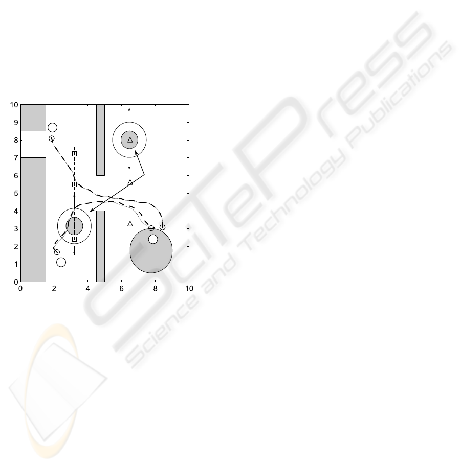
Fig. 5 shows by the dotted line as outcome of the
MPC algorithm the motion of the service robot from
the kitchenette (1) to the table (2) and further to the
refrigerator (3). The underlying map represents the
kitchen in 2D and is used for the localization of the
robot. For three time stamps t
1
,t
2
, and t
3
the posi-
tions of the robot and the two persons are marked by
a circle, and by a square / triangle respectively. The
dash-dotted lines mark the motion of the two persons.
2
People in motion
with safety margin
1
3
t
0
t
0
t
0
t
1
t
1
t
1
t
2
t
2
t
2
Figure 5: Trajectories of the robot moving between kitch-
enette (1), table (2), and refrigerator (3).
For each varying goal positions, the knowledge
base is filled with information on goal-attaining
strategies for future use. Employing the knowledge
base reduces the calculation time essentially. The ser-
vice scenario is simulated in the Player/Stage/Gazebo
(PSG) environment.
7 CONCLUSIONS AND
OUTLOOK
The aim of the presented concept is to provide an ar-
chitecture by which the combination of control meth-
ods applied to hybrid systems, techniques from artifi-
cial intelligence, and vertical decomposition of tasks
is realized. Simultaneously, the approach intends to
cover the whole perception-reasoning-action loop of
an autonomous system that has to make decisions for
goal-oriented behavior in new situations. While the
considered example is quite simple, it illustrates the
mechanism of task decomposition and improves ef-
ficiency of computing suitable control trajectories by
the use of machine learning techniques.
Current work is focussed on extending the plan-
ning hierarchy to different learning and control algo-
rithms.
ACKNOWLEDGEMENTS
Partial financial support of this investigation by the
DFG within the Cluster of Excellence Cognition for
Technical Systems is gratefully acknowledged.
REFERENCES
Barto, A. G. and Mahadevan, S. (2003). Recent advances
in hierarchical reinforcement learning. Discrete Event
Dynamic Systems, 13(1-2):41–77.
Broy, M. and Stoelen, K. (2001). Specification and De-
velopment of Interactive Systems: Focus on Streams,
Interfaces, and Refinement. Springer.
Galindo, C., Fernandez-Madrigal, J., and Jesus, A. G.
(2007). Multiple abstraction hierarchies for mobile
robot operation in large environments. Studies in
Computational Intelligence, Springer.
Haberl, W., Tautschnig, M., and Baumgarten, U. (2008).
Running COLA on Embedded Systems. In Proceed-
ings of The International MultiConference of Engi-
neers and Computer Scientists 2008.
Henzinger, T. (1996). The theory of hybrid automata. In
Proceedings of the 11th Annual IEEE Symposium on
Logic in Computer Science (LICS ’96), pages 278–
292.
LaValle, S. M. (2006). Planning Algorithms. Cambridge
University Press.
Morari, M., Garcia, C., and Prett, D. M. (1989). Model
predictive control: Theory and practice-A survey. Au-
tomatica, 25(3):335–348.
Nau, D. S., Smith, S. J. J., and Erol, K. (1998). Control
strategies in HTN planning: Theory versus practice.
In AAAI/IAAI, pages 1127–1133.
Stursberg, O. (2006). Supervisory control of hybrid systems
based on model abstraction and refinement. Journal
on Nonlinear Analysis, 65(6):1168–1187.
Takadama, K. and Fujita, H. (2004). Lessons learned from
comparison between q-learning and sarsa agents in
bargaining game. In Conference of North American
Association for Computational Social and Organiza-
tional Science, pages 159–172.
EFFICIENT PLANNING OF AUTONOMOUS ROBOTS USING HIERARCHICAL DECOMPOSITION
267