
SLAM AND MULTI-FEATURE MAP BY FUSING 3D LASER AND
CAMERA DATA
Ayman Zureiki, Michel Devy and Raja Chatila
CNRS, LAAS, 7 avenue du Colonel Roche, F-31077 Toulouse, France
Universit´e de Toulouse, UPS, INSA, INP, ISAE, LAAS-CNRS, F-31077 Toulouse, France
Keywords:
Data Fusion, SLAM, Heterogeneous Maps.
Abstract:
Indoor structured environments contain an important number of planar surfaces and line segments. Using
these both features in a unique map gives a simplified way to represent man-made environments. Extracting
planes and lines by a mobile robot requires more than one sensor: a 3D laser scanner and a camera can
be a good equipment. The incremental construction of such a model is a Simultaneous Localisation And
Mapping (SLAM) problem: while exploring the environment, the robot executes motions; from each position,
it acquires sensory data, extracts perceptual features, and simultaneously, performs self-localisation and model
update. First, the 3D range image is segmented into a set of planar faces which are used as landmarks. Next,
we describe how to extract 2D line landmarks by fusing data from both sensors. Our stochastic map is of
heterogeneous type and contains plane and 2D line landmarks. At first, The SLAM formalism is used to build
a stochastic planar map, and results on the incremental construction of such a map are presented, further on,
heterogeneous map will be constructed.
1 INTRODUCTION
Simultaneous Localisation and Mapping is a funda-
mental technology for autonomous mobile robots. A
robot needs a description of his environment. Maps
are required for self-localisation, for motion planning,
etc. In this article, we deal with the on line learning of
such maps for a structured (man-made) environment
supposed unknown.
Using the SLAM algorithm, the robot performs
a complex process, including the execution of mo-
tions, the acquisition of sensory data, data associa-
tion between these sensory data and the current world
model, estimation of the robot pose using these as-
sociations and finally, the incremental construction of
the map. It has to take into account many geomet-
ric constraints, and many sources of errors. Essen-
tially, the robustness to achieve this task depends on
the robot capabilities to extract pertinent information
(called Landmarks) from sensory data coming from
embedded sensors. The robot starts up from an ini-
tial position without any a priory knowledge about
landmarks: by use of relative measurements on land-
marks, the robot estimates its pose and poses of the
landmarks in an absolute frame, generally selected as
the initial pose of the robot. When moving, the robot
updates the landmark map and exploits it to produce
an estimate of its pose. The delivered map can be of
intuitive representation for humans or not. In the liter-
ature we can find three main types of maps. Topolog-
ical, metric and hybrid maps. A topological map can
be seen as an abstract representation describing re-
lations between environment areas (typically, rooms
or corridors). Such maps are well adapted for route
planning, the selection of the best strategy for mo-
tions between areas. Their main drawback is the ab-
sence of geometric information. On the contrary, a
metric map provides a (detailed) geometric represen-
tation of the environment; it gives explicit metric in-
formation (lengths, widths, positions, etc.), generally
expressed with respect to a global reference frame.
The third class is the Atlas which is a Hybrid metri-
cal/topological approach to SLAM capable to achieve
efficient mapping of large-scale environments (Bosse
et al., 2003).
SLAM has been an active research topic for more
than twenty years; many works from Durrant-White,
Tardos, Nebot, Dissanayake, Feder, Leonard, New-
man, Rencken...aim to develop generic tools, based
on the formalism of stochastic maps proposed by
(Smith et al., 1990). The majority of these works have
focused on the estimation methods required in order
to maintain estimates of the robot pose and of land-
mark attributes in a consistent stochastic map. The
extended Kalman Filter (EKF) was initially proposed
as a mechanism that allows the incremental fusion of
101
Zureiki A., Devy M. and Chatila R. (2008).
SLAM AND MULTI-FEATURE MAP BY FUSING 3D LASER AND CAMERA DATA.
In Proceedings of the Fifth International Conference on Informatics in Control, Automation and Robotics - RA, pages 101-108
DOI: 10.5220/0001500701010108
Copyright
c
SciTePress

information acquired by the robot; later, other meth-
ods have been exploited successfully (information fil-
ter, particle filter etc.), especially in the FastSLAM
method, proposed by (Thrun et al., 1998). A well de-
tailed state of the art can be found in (Durrant-Whyte
and Bailey, 2006).
These approaches have been validated mainly by
constructing 2D representations (2D segment maps
etc.) of indoor environment from laser data acquired
typically by SICK range finders. Recently, 3D SLAM
draws attention. (Takezawa et al., 2004) describes a
SLAM framework based on 3D landmarks. (Jung,
2004) constructs a 3D map from interest points in
outer environment using stereo vision data; (Sola
et al., 2005) builds such maps using only monocu-
lar vision. These sparse representations allow essen-
tially the robot to locate itself. Our work is focused
on the construction of surface model in indoor envi-
ronment, where many planar surfaces (ceiling, floor,
walls, doors etc.) can be used as landmarks. Our
goal is to produce a geometric stochastic map made
of 3D planar features. In the same area, let us cite
the preliminary contributionof (Nashashibi and Devy,
1993), with an off line validation from a limited num-
ber of range images, and the works of (Thrun et al.,
2000) based on the exploitation of two laser ranger
finders to acquire measurements on horizontal and
vertical planes and to produce a dense model of 3D
points, from which a mesh can be constructed a pos-
teriori. (Abuhadrous et al., 2004) developed a sim-
ilar approach to model urban sites using GPS to lo-
calise the vehicle. Finally using only monocular vi-
sion, planes are extracted by using homographs and
fused by a SLAM approach in (Silveira et al., 2006).
While the algorithm of SLAM is well known and
studied, using new sensors and robust features extrac-
tion remains an open topic. Sensors’ data fusion is
an interesting approach to overcome the deficiency of
each sensor and to obtain more sophisticated and ac-
curate results. In this paper,we present a noveltype of
Heterogeneous multi-feature metric maps. Our map
contains two types of features: 3D Planes and 2D
lines attached to these planes. While planes are ex-
tracted from 3D point cloud issue from 3D laser scan-
ner, the 2D lines are extracted by fusing data from the
laser scanner with image data from a camera.
In the section 3 we give details about features ex-
traction: planar features from range images, and 2D
line segments from both laser and camera data. Then
in section 4, we define our heterogeneous map which
contains plane and 2D line landmarks. Next in section
5 we adapt the slam algorithm for both of used fea-
tures. Finally in section 6, experimental results using
our mobile robot (Jido) are discussed, before summa-
rizing our contribution and presenting current works
in section 7.
2 NOTATION
As we use many reference frames and two features, it
is useful to summarise used notations. Let R
1,2
and
t
1,2
be the rotation matrix and the translation vector
from reference frame 1 to frame 2. For a 3D point
represented by P
1
in the frame 1 and by P
2
in the
frame 2, we have:
P
1
= [x
1
y
1
z
1
]
T
(1)
P
1
= R
1,2
P
2
+ t
1,2
(2)
Used Frames.
• R
sk
: SICK frame.
• R
c
: camera frame.
• R
r
: robot frame.
• R
w
: global (world) frame.
• R
p
: plane landmark local frame.
The transformations between these frames are
given by the following matrices and vectors:
• R
r,sk
and t
r,sk
: from robot to SICK frames.
• R
r,c
and t
r,c
: from robot to camera frames.
• R
w,r
and t
w,r
: from world to robot frames.
• R
w, p
and t
w, p
: from world to plane landmark
frames.
The robot pose is defined by (x
v
, y
v
, θ
v
)
T
in the
world frame.
3 FEATURES EXTRACTION
We detail in this section the extraction of used land-
marks from sensory data.
3.1 Plane Extraction
3D laser scanner provides range images with thou-
sands of 3D points. Segmenting the range image
means how to divide it into features, i.e. how to bind
each point with a label identifying to which feature it
belongs, so that points of the same plane have all the
same label. For a mobile robot, segmenting range im-
ages is a difficult topic, because the robot does not
know a priori what is seen in the scene; moreover
segmentation process must be robust in presence of
ICINCO 2008 - International Conference on Informatics in Control, Automation and Robotics
102

non-planar or non static objects and in spite of mea-
surements’ noises. The planar segmentation has been
well studied in computer graphics in order to perform
real-time rendering of complex models (Heckbert and
Garland, 1997). A major difference exists between
robotics and computer graphics. Data in robotics are
issued from sensors and hence they are erroneous,
while models in computer graphic are supposed to be
without errors.
(H¨ahnel et al., 2003) proposed a simplification
algorithm adapted to robotic context. They extract
planes by using an approach of type region-growing
by starting from an arbitrary point, then try to enlarge
the region in all directions. (Weingarten, 2006) pro-
posed some improvementto this algorithm by starting
region seed from the most flat point in the cloud (min-
imum local error), and by profiting from the struc-
ture of the range image to simplify the research of
neighbour points. Our approach is based on these two
works, with some differences in the choice of plane’s
parameters and the method of their estimation.
3.1.1 Plane Equation
A plane can be represented by three parameters: the
distance from the origin ρ and two angles. Let ϕ be
the angle between the projection of the plane normal
on the OXY plane and the axis
−→
OX, and let ψ be the
angle between the plane normal with the axis
−→
OZ. The
plane equation is then:
cosϕ sinψ x+ sinϕ sinψ y + cosψ z+ ρ = 0 (3)
The vector (ρ ϕ ψ)
t
will be used as the minimal
parametric representation of a plane.
3.1.2 Estimation Process
Kalman Filter is a recursive estimator : to estimate
the current state, only the previous state and the ac-
tual measurements are required. The observation his-
tory is not needed. In the Extended Kalman Filter
(EKF), the dynamic and observation models could be
non-linear functions. To estimate the parameters of a
plane we use and EKF. We consider that each point
belonging to a plane as an observation of this plane.
We detail the estimation process in (Zureiki and Devy,
2008).
3.1.3 Choice of Plane Landmark Local
Reference
Let P be a plane landmark defined by its parameters
(ρ
w
, ϕ
w
, ψ
w
) in the global frame R
w
. We are looking
for a orthonormal frame of this plane. We choose the
projection of the origin O
w
on the plane P as an origin
O
p
of local frame, and the axis Z
p
to be parallel to the
normal vector n. We need to choose the axis X
p
. Let
−→
i
w
,
−→
j
w
,
−→
k
w
be the unit vectors of axes O
w
X, O
w
Y, O
w
Z
respectively, and
−→
i
p
,
−→
j
p
,
−→
k
p
be unit vectors of wanted
axes O
p
X
p
, O
p
Y
p
, O
p
Z
p
respectively.
−→
i
p
=
sinϕ
w
−cosϕ
w
0
T
(4)
This vector can be interpreted as the unit vector
of direction of the intersection line between the plane
P and the plane Z = 0 (if they are not parallel). The
rotation matrix from global to the local references is:
R
w, p
=
sinϕ
w
cosϕ
w
cosψ
w
cosϕ
w
sinψ
w
−cosϕ
w
sinϕ
w
cosψ
w
sinϕ
w
sinψ
w
0 −sinψ
w
cosψ
w
(5)
and the translation vector is:
t
w, p
= ρ
w
cosϕ
w
sinψ
w
sinϕ
w
sinψ
w
cosψ
w
(6)
3.2 2D Line Landmark Extraction
By mean of a camera we extract 2D segments in the
image. These segments can be interpreted as the pro-
jection of 3D Lines (or more generally Planes) onto
the image plane. The first idea to come is to use
the 3D Lines as a second type of landmarks in the
stochastic map. To define a 3D line we need to de-
fine two planes. Using the camera, we can obtain one
of them, so we need to use the 3D laser to define the
other plane. By fusing the data of both sensors we
can extract 3D lines in the scene. For representation
reasons, we will consider the 3D line as 2D line at-
tached to a holding plane. The holding plane is define
by the laser data (as describe in 3.1). This represen-
tation seems reasonable, because the 3D line may be
either a corner (intersection of two planes) or the bor-
ders of a poster fixed on a wall for example, and in
both cases a 2D line in the local plane frame is suffi-
cient to totally define it. As a result, we need to add to
the map only the parameters defining a 2D line in the
plane landmark frame. Therefore, the second type of
Landmarks for us is a 2D Line attached to a Plane
Landmark.
3.2.1 Advantages of Data Fusion
Data fusion is the technique of combining data from
multiple sensors or information from differentsources
to achieve more specific inferences than could be
SLAM AND MULTI-FEATURE MAP BY FUSING 3D LASER AND CAMERA DATA
103

reached by using a single independent sensor. Fused
data provide several advantages over single sensor
data (Hall and Llinas, 2001). First, if several identical
sensors are used, combining the observations will re-
sult in an improved estimate of the observed quantity.
A statistical advantageis gained by adding Nindepen-
dent observations. The same result could be obtained
also by combining N observations from an individ-
ual sensor. A second advantage involves using the
relative placement of multiple sensors to improve the
observation process. For example, two sensors (cam-
era) that observe the same object can coordinate to
determine the 3D position of the object by triangula-
tion (stereo vision). A third advantage of using mul-
tiple sensors is improved observability. For a robot
equipped by a 3D laser scanner and a camera, the
laser scanner can accurately determine the range of
an obstacle (wall for example), camera can determine
the visual properties of the obstacle but can not deter-
mine its range. By using the camera we can recognise
whether the robot is in front of a wall or a closed door.
If these two observations are correctly associated, the
combination of the two sensors provides a better lo-
calisation than could be obtained by either of the two
independent sensors.
In our work, we use the 3D laser scanner to extract
planes from the 3D range images. A camera is used to
extract 2D lines in images. By combining the camera-
laser data, we define a new landmark as : 2D line
attached to a 3D plane landmark. This 2D line land-
mark could be seen as graduations on a ruler, while
the ruler defines the plane in the 3D space, the gradua-
tions on it define more information with respect to the
ruler plane. So with these two landmarks, a robot can
be localised with respect to a plane and with respect
to the graduations (2D line landmarks) on this plane.
The importance of such landmarks can be more illus-
trated in a long corridor formed with two walls (and
eventually with closed doors). Using only plane land-
marks will lead to only two parallel planes. Using a
camera to extract 2D lines in the image (may be bor-
ders of a poster fixed on the wall, or the borders of a
door), and fusion laser-camera data will provide a 2D
line fixed on the wall in a precise position. The robot
will be localised with respect to both plane and line:
the plane will help to find latitude information, while
the 2D line will add longitude information.
3.2.2 2D Line Extraction in Images
We use a traditional method of line extraction in im-
ages. It begins by a Canny filter to extract the contour,
then we use a polygonal approximation to estimate
the line passing through adjacent contour points. A
phase of post processing is necessary to merge simi-
lar segments and to remove very small ones.
3.2.3 Interpretation Plane
For a line segment l
I
in the image, the associated In-
terpretation plane is the plane passing through this
2D line and the centre of projection (viewpoint) of
the camera. The normal vector of this plane can be
calculated only based on intrinsic parameters of the
camera (α
u
, α
v
, u
0
, v
0
) and the data image of the seg-
ment. In fact, let (δ
I
, γ
I
) be the 2D line parameters
of the infinite line holding the 2D segment l
I
, where
γ
I
is the angle with the axis u and δ
I
is the distance
from the origin. The 2D line equation is in the image
reference frame:
cosγ
I
u+ sinγ
I
v− δ
I
= 0 (7)
Then using camera coordinates:
cosγ
I
(α
u
x
c
z
c
+ u
0
) + sinγ
I
(α
v
y
c
z
c
+ v
0
) − δ
I
= 0 (8)
we obtain:
α
u
cosγ
I
x
c
+ α
v
sinγ
I
y
c
+
+(−δ
I
+ u
0
cosγ
I
+ v
0
sinγ
I
) z
c
= 0
(9)
The normal vector in the camera reference frame
is given by:
n
c
=
α
u
cosγ
I
α
v
sinγ
I
−δ
I
+ u
0
cosγ
I
+ v
0
sinγ
I
(10)
and the distance to the origin in camera frame d
c
= 0.
The interpretation plane in the robot, world, plane
landmark frames is noted respectively by: (n
r
, d
r
),
(n
w
, d
w
) and (n
p
, d
p
). We note also:
n
c
= [n
c,x
n
c,y
n
c,z
]
T
n
r
= [n
r,x
n
r,y
n
r,z
]
T
n
w
= [n
w,x
n
w,y
n
w,z
]
T
n
p
= [n
p,x
n
p,y
n
p,z
]
T
(11)
3.2.4 The 2D Line in the Plane Landmark
Frame
The interpretation plane in the plane landmark frame
is given by:
n
p
= R
T
w, p
R
w,r
R
r,c
n
c
d
p
= d
c
− t
T
r,c
R
r,c
n
c
− t
T
w,r
R
w,r
R
r,c
n
c
+t
T
w, p
R
w,r
R
r,c
n
c
(12)
ICINCO 2008 - International Conference on Informatics in Control, Automation and Robotics
104
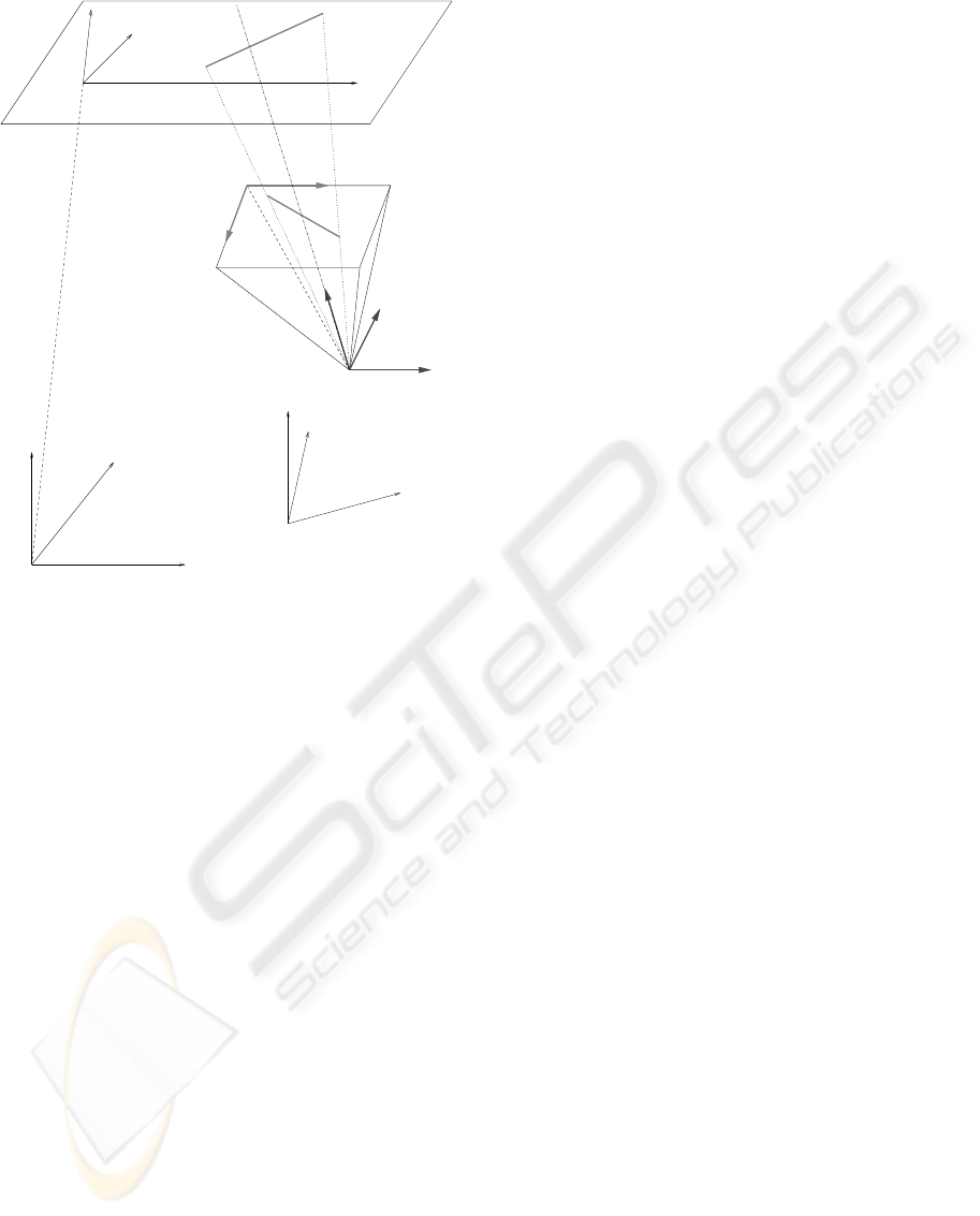
Z
c
Y
p
X
p
X
c
Y
c
O
c
Y
i
X
w
Z
w
O
w
O
r
X
r
Y
r
Z
r
Z
p
−→
n
X
i
Y
w
O
p
Figure 1: A 2D Segment in image and its corresponding 2D
Line Landmark attached to the Plane Landmark.
Hence, we obtain the normal vector and the dis-
tance from the origin (n
p
, d
p
) of the interpretation
plan in the plane landmark frame. The 3D line of
the intersection between the interpretation plane with
the plane z
p
= 0 can be seen as 2D line in the plane
O
p
X
p
Y
p
, therefore, the 2D line landmark equation in
the plane landmark frame is:
n
x, p
x
p
+ n
y, p
y
p
+ d
p
= 0 (13)
4 THE STOCHASTIC MAP
Indoor environment can be considered (in a simpli-
fied way) as a set of planar surfaces which we choose
as landmarks for the SLAM algorithm. Attached to
these plane surfaces we consider another type of land-
marks: the 2D lines.
The SLAM algorithm maintains a representation
of both the environment state and the robot state. Dur-
ing the robot displacement, it uses its sensors to ob-
serve the surrounding landmarks. The system state at
time k, X(k), is composed of the robot state X
v
, and of
n
f
vectors describing the observed landmarks, X
i
(k),
i = 1, . . . , n
f
.
X(k) = [X
W
v
X
1
. . . X
n
f
]
T
(14)
where X
i
is the state of a landmark i either in the
global frame R
W
if it is a plane landmark or in hold-
ing plane frame if it is a 2D line landmark. We can
rearrange the system state vector so that we group the
states of landmarks in one term X
m
(k) :
X(k) =
X
W
v
X
W
m
(15)
The robot state at time k can be determined by its
position and orientation in the space. The robot state
vector is defined by: X
v
(k) = [x
v
(k), y
v
(k), θ
v
(k)]
T
.
Each planar surface (wall, ceiling, floor etc.), is con-
sidered as an infinite plane defined by three parame-
ters X
π, j
(k) = [ρ
j
(k), ϕ
j
(k), ψ
j
(k)]
T
. Each 2D Seg-
ment is considered as an infinite line in the holding
plane landmark and is defined by means of two pa-
rameters X
L,i
(k) = [δ
i
(k), γ
i
(k)]
T
. Of course, a plane
landmark can contain many 2D line landmarks, but a
2D line landmark can not exist alone without a hold-
ing plane landmark. Our stochastic map is then an
heterogeneous map, as it has two types of landmarks.
5 THE SLAM ALGORITHM
We detail the main steps in the SLAM algorithm
adapted to the used landmarks.
5.1 Prediction
The prediction phase of the extended Kalman filter
uses the dynamic model of the robot to produce an
estimate of the robot motion X
v
(k|k − 1), at time k
knowing all the information until time k− 1, and the
control input u(k):
ˆ
X
v
(k|k − 1) = f(
ˆ
X
v
(k− 1|k − 1), u(k)) (16)
We can write the prediction phase of the filter as:
ˆ
X
v
(k|k − 1)
ˆ
X
m
(k|k − 1)
=
f(
ˆ
X
v
(k−1|k− 1), u(k))
ˆ
X
m
(k−1|k− 1)
(17)
The covariance matrix must propagate through the
robot model in this phase. The extended Kalman filter
linearise the propagation of the uncertaintyaround the
current estimate
ˆ
X(k− 1|k−1) by using the Jacobean
∇
X
f(k) of f at
ˆ
X(k− 1|k− 1). Q(k) is the covariance
of the error.
P(k|k−1) = ∇
X
f(k) P(k−1|k−1) ∇
X
f
T
(k) +Q(k) (18)
SLAM AND MULTI-FEATURE MAP BY FUSING 3D LASER AND CAMERA DATA
105

For the SLAM algorithm, this phase can be sim-
plified thanks to the hypothesis that the landmarks
are fix. This let us reduce the calculation complex-
ity of the prediction covariance to only the calcula-
tion of covariance of robot pose and cross-covariance
between the robot and the map (Williams, 2001).
5.2 Observation of 3D Plane
Landmarks
For plane landmarks, the innovation function is:
ν = Z(k) −
ˆ
Z(k|k− 1) (19)
where:
• Z(k) : the current measurement, i.e. the ex-
tracted planes from the 3D range image in the
robot frame, with a covariance matrix R(k).
•
ˆ
Z(k|k − 1) : estimation of measurement, i.e. how
the plane landmarks in the stochastic map are po-
sitioned with respect to the current robot pose in
robot frame. Hence the measurement estimation
is a function of the predicted state of the system:
ˆ
Z(k|k− 1) = h(
ˆ
X(k|k− 1)) (20)
Measurement Estimation. In the case of plane/plane
fusion: Let (ρ
w
, ϕ
w
, ψ
w
) and (ρ
r
, ϕ
r
, ψ
r
) be the param-
eters of a plane in the global and robot frame respec-
tively. For a robot moving on horizontal floor, the
relation between a plane parameters in the global and
robot frame is:
ρ
r
= ρ
w
− cosϕ
w
sinψ
w
x
v
−sinϕ
w
sinψ
w
y
v
ϕ
r
= ϕ
w
− θ
v
ψ
r
= ψ
w
(21)
Then, the observation prediction of a plane land-
mark relatively to the robot frame:
ˆ
Z(k|k− 1) =
ˆ
ρ
r
(k|k − 1)
ˆ
ϕ
r
(k|k − 1)
ˆ
ψ
r
(k|k − 1)
(22)
5.3 Observation of 2D Line Landmarks
The procedure of updating the stochastic map is the
following: First we update the plane landmarks using
only the 3D laser data. Then, we update the 2D line
landmarks on each plane.
Innovation Function. With 2D line landmarks at-
tached to plane landmarks, the innovation function is
written:
ν = Z(k) −
ˆ
Z(k|k− 1) (23)
where:
• Z(k) : the current measurement of the 2D line
landmark attached to a plane. In reality, we obtain
this measurement by fusing 3D laser and camera
data. Hence the current measurement is a function
of the system state. This measurement is in plane
landmark local frame.
Z(k) = h(
ˆ
X(k|k − 1), Image) (24)
•
ˆ
Z(k|k − 1) : estimation of measurement, i.e. how
the 2D line landmarks attached to a plane land-
mark are positioned in the local plane frame. In
fact, the 2D line landmarks are fix with respect to
the plane holding them
ˆ
Z(k|k − 1) =
ˆ
Z(k− 1|k − 1) (25)
Innovation Covariance Matrix.
S(k) = P
ii
(k|k − 1) + R(k) (26)
where P
ii
(k|k − 1) is the covariance matrix of the
2D line landmark i, and R(k) is the covariance matrix
of the current measurement. See the previous note,
we write:
Z(k) = h(
ˆ
X
v
(k|k − 1),
ˆ
X
j
(k|k − 1), X
I
(k)) (27)
where
ˆ
X
j
(k|k−1) is the predicted state of holding
plane landmark, and X
I
(k) is the camera data (image
2D line parameters) with a covariance matrix Λ
I
.
With ∇
v
h, ∇
j
h and ∇
I
h are the Jacobians of the
function h with respect to the robot, plane landmark j
and 2D line in Image l
I
respectively, we have:
R(k) = ∇
v
h P
vv
∇
v
h
T
+ ∇
v
h P
vj
∇
j
h
T
+∇
j
h P
j j
∇
j
h
T
+ ∇
j
h P
T
vj
∇
v
h
T
+∇
I
h Λ
I
∇
I
h
T
(28)
In this last equation, we identify clearly the role
of camera data which are not correlated to laser data.
This allows us to justify our choice for 2D Line Land-
marks attached to plane landmark. In spite of the intu-
itive idea that the 2D line landmark will be correlated
to the plane landmark holding it, a part of data (cam-
era data) defining the 2D line is not correlated with
the data defining the holding plane. This proves that
the two landmarks are not correlated.
ICINCO 2008 - International Conference on Informatics in Control, Automation and Robotics
106
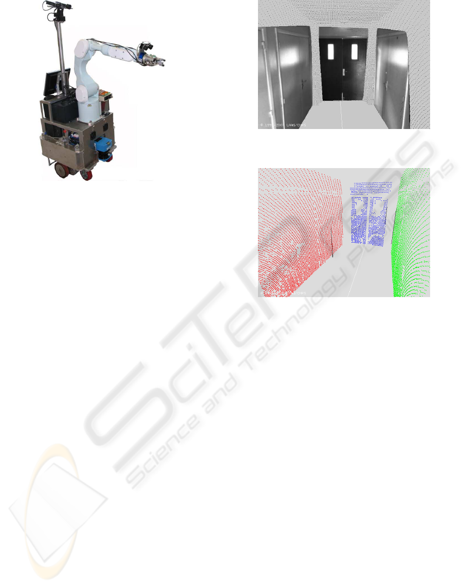
Figure 2: The mobile robot Jido.
5.4 Update
Once an observation is associated to a landmark in the
map, the estimate of system state can be updated us-
ing the gain matrix W(k). The gain matrix provides
a weighted sum of the prediction and observation,
and is calculated based on the innovation covariance
matrix S(k), and the prediction of covariance matrix,
P(k|k − 1). The weighting factor is proportional to
P(k|k − 1) and inversely proportional to innovation
covariance (Smith et al., 1990). This can be used to
update the system state vector
ˆ
X(k|k) and its covari-
ance matrix P(k|k).
ˆ
X(k|k) =
ˆ
X(k|k − 1) + W(k)ν(k) (29)
P(k|k) = P(k|k− 1) − W(k) S(k)W
T
(k) (30)
where
W(k) = P(k|k− 1) ∇
X
h
T
S
−1
(k) (31)
6 IMPLEMENTATION AND
RESULTS
We used in the experimentsour robot JIDO (figure 2).
It has (among other sensors) a SICK LMS-200 Range
finder fixed on a rotating axis installed ahead, a stereo
rig on a pan/tilt.
The 3D scanner laser has an angular resolution
of 0.5
◦
, with a field of view of 180
◦
which gives 361
points per scan. For the rotation of scanner around
the horizontal axis, we choose to make steps of 0.01
Rad (≈ 0.57
◦
) and to rotate the scanner between
−0.3 Rad (≈ −17
◦
) and 1.4 Rad (≈ 80
◦
), which
Figure 3: Experimental Results.
Figure 4: Plane Landmarks and some 2D Line Landmarks
attached to them.
includes 171 scans. The produced range image is
composed of 171 ∗ 361 = 61731 points. The left
camera of the stereo rig is used to acquire images.
The robot did a tour in our laboratory, it moves
and halts, takes measurements, then it advances
again. It has made a tour in a corridor and did a
half turn to return to the point of departure, making
in all 12 displacements. We implement a classical
EKF SLAM algorithm. The incremental construction
of the map of the corridor is illustrated (partially)
in the figure 3, where we choose to print only the
points belonging to each planar facet in the stochastic
map. The points of each plane are assembled from
the successive fused planes’ points. The texture
was mapped onto the planes using a homography
transformation from initial image and a virtual image
placed on the plane.
Figure 4 represent an image with the extracted 2D
line segments, and figure 5 represents 3D planes ex-
tracted from laser scanner and on which are attached
to some 2D line landmarks coming from the fusion
algorithm explained in this article. For now only
plane landmarks are added to the stochastic map, the
addition of 2D line landmarks is under construction.
SLAM AND MULTI-FEATURE MAP BY FUSING 3D LASER AND CAMERA DATA
107
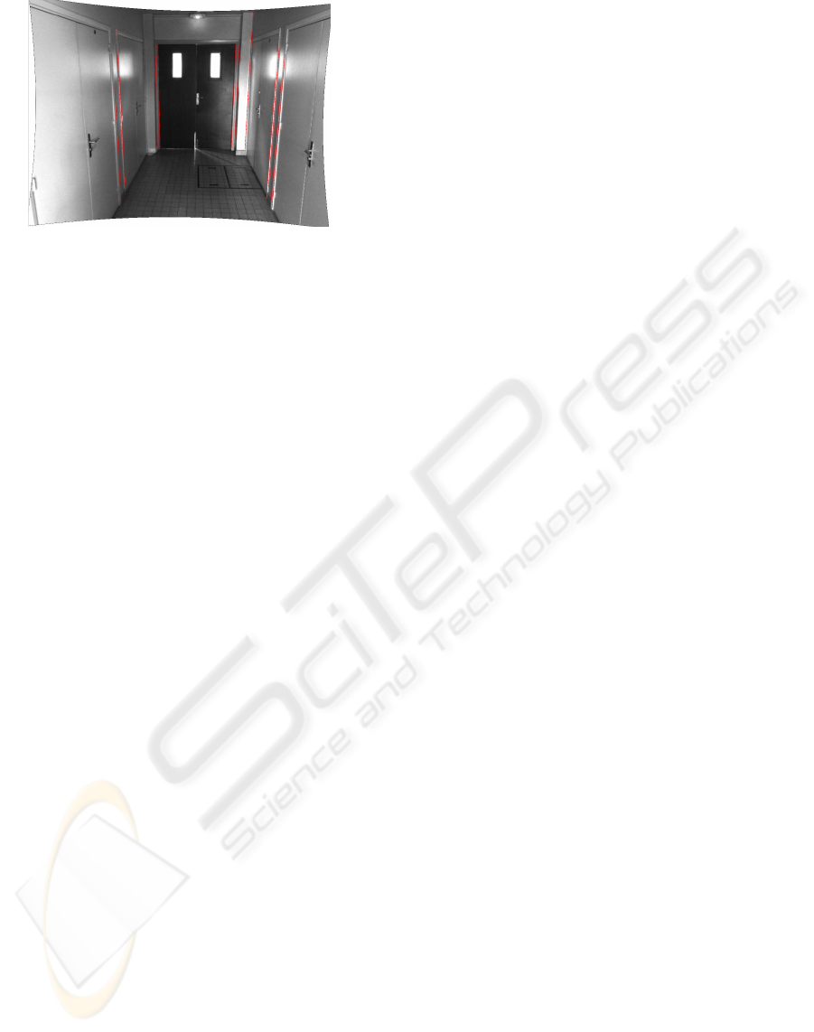
Figure 5: Image with the extracted 2D line Segments.
7 CONCLUSIONS
This paper has described an heterogeneous 3D
stochastic map building using a SLAM method. The
map has 3D plane landmarks and 2D line landmarks.
Features extraction is detailed with the emphasis on
the fusion of laser and camera data to obtain 2D line
landmarks. Preliminary results on 2D line landmarks
was presented, as well as a map reconstructed only
with planar landmarks. The current work is to achieve
the building of the heterogeneous map.
Adding 2D lines to planes has two major bene-
fits: make the map more rich for navigation, and at
the same time enforce the phase of data association of
plane landmarks.
Due to the acquisition time using the laser scanner
sensor, the robot must stop during the scanning: the
same method will be applied with continuousacquisi-
tion made from a PMD sensor (Swiss Ranger from the
CSEM company) mounted on the mast of our robot.
REFERENCES
Abuhadrous, I., Ammoun, S., Nashashibi, F., Goulette, F.,
and Laurgeau, C. (2004). Digitizing and 3d modelling
of urban environments using vehicle-borne laser scan-
ner system. In Proc. IEEE/RSJ International Confer-
ence on Intelligent Robots and Systems (IROS).
Bosse, M., Newman, P., Leonard, J., Soika, M., Feiten, W.,
and Teller, S. (2003). An atlas framework for scalable
mapping. In International Conference on Robotics
and Automation (ICRA03), pages 1899–1906.
Durrant-Whyte, H. and Bailey, T. (2006). Simultaneous Lo-
calization and Mapping (SLAM): Part I & II. IEEE
Robotics & Automation Magazine.
H¨ahnel, D., Burgard, W., and Thrun, S. (2003). Learning
compact 3d models of indoor and outdoor environ-
ments with a mobile robot. Robotics and Autonomous
Systems.
Hall, D. L. and Llinas, J., editors (2001). Handbook of Mul-
tisensor Data Fusion. CRC Press LLC.
Heckbert, P. S. and Garland, M. (1997). Survey of polyg-
onal surface simplification algorithms. Technical re-
port, Carnegie-Mellon Univ.
Jung, I. K. (2004). Simultaneous localization and mapping
in 3D environments with stereovision. PhD thesis, In-
stitut National Polytechnique de Toulouse, France.
Nashashibi, F. and Devy, M. (1993). 3d incremental model-
ing and robot localization in a structured environment
using a laser range finder. In Proc. IEEE International
Conference on Robotics and Automation (ICRA).
Silveira, G., Malis, E., and Rives, P. (2006). Real-time ro-
bust detection of planar regions in a pair of images. In
Proc. IEEE/RSJ International Conference on Intelli-
gent Robots Systems, Beijing, China.
Smith, R., Self, M., and Cheeseman, P. (1990). Estimat-
ing uncertain spatial relationships in robotics. Au-
tonomous robot vehicles, pages 167–193.
Sola, J., Monin, A., Devy, M., and Lemaire, T. (2005).
Undelayed initialization in bearing only slam. In
Proc. IEEE/RSJ International Conference on Intelli-
gent Robot and Systems (IROS), pages 2751–2756.
Takezawa, A., Herath, D. C., and Dissanayake, G. (2004).
Slam in indoor environments with stereo vision. In
Proceedings of 2004 IEEE/RSJ International Confer-
ence on Intelligent Robots and Systems.
Thrun, S., Burgard, W., and Fox, D. (1998). A probabilistic
approach to concurrent mapping and localization for
mobile robots. Machine Learning, 31(1-3):29–53.
Thrun, S., Fox, D., and Burgard, W. (2000). A real-time
algorithm for mobile robot mapping with application
to multi robot and 3d mapping. In Proc. IEEE In-
ternational Conference on Robotics and Automation
(ICRA).
Weingarten, J. (2006). Feature-based 3D SLAM. PhD the-
sis,
´
Ecole Polytechnique F´ed´erale de Lausanne.
Williams, S. (2001). Efficient Solutions to Autonomous
Mapping and Navigation Problems. PhD thesis, The
University of Sydney.
Zureiki, A. and Devy, M. (2008). Slam and data fusion
from visual landmarks and 3d planes. In Proc. the
17th IFAC World Congress.
ICINCO 2008 - International Conference on Informatics in Control, Automation and Robotics
108
