TWO-SIDED ASSEMBLY LINE

Estimation of Final Results

Waldemar Grzechca

Institute of Automatic Control, The Silesian University of Technology, ul.Akademicka 16, 44-100 Gliwice, Poland

Keywords: Assembly line balancing, Two-sided structure, Line time, Line efficiency, Smoothness index.

Abstract: The paper considers simple assembly line balancing problem and two-sided assembly line structure. In the

last four decades a large variety of heuristic and exact solutions procedures have been proposed to balance

one-sided assembly line in the literature. Some heuristic were given to balance two-sided lines, too. Some

measures of solution quality have appeared in line balancing literature: balance delay (BD), line efficiency

(LE), line time (LT) and smoothness index (SI). These measures are very important for estimation the

balance solution quality. Author of this paper modified and discussed the line time and smoothness for two-

sided assembly line. Some problems, which appeared during evaluations, are mentioned.

1 INTRODUCTION

The manufacturing assembly line was first

introduced by Henry Ford in the early 1900’s. It was

designed to be an efficient, highly productive way of

manufacturing a particular product. The basic

assembly line consists of a set of workstations

arranged in a linear fashion, with each station

connected by a material handling device. The basic

movement of material through an assembly line

begins with a part being fed into the first station at a

predetermined feed rate. A station is considered any

point on the assembly line in which a task is

performed on the part. These tasks can be performed

by machinery, robots, and/or human operators. Once

the part enters a station, a task is then performed on

the part, and the part is fed to the next operation. The

time it takes to complete a task at each operation is

known as the process time (Sury, 1971). The cycle

time of an assembly line is predetermined by a

desired production rate. This production rate is set so

that the desired amount of end product is produced

within a certain time period (Baybars, 1986). For

instance, the production rate might be set at 480

parts per day. Assuming an eight-hour shift, this

translates into a requirement of 60 parts per hour (1

part per minute) being produced by the assembly

line. In order for the assembly line to maintain a

certain production rate, the sum of the processing

times at each station must not exceed the stations’

cycle time (Fonseca et. al, 2005). If the sum of the

processing times within a station is less than the

cycle time, idle time is said to be present at that

station (Erel, Erdal and Sarin, 1998). One of the

main issues concerning the development of an

assembly line is how to arrange the tasks to be

performed. This arrangement may be somewhat

subjective, but has to be dictated by implied rules set

forth by the production sequence (Kao, 1976). For

the manufacturing of any item, there are some

sequences of tasks that must be followed. The

assembly line balancing problem (ALBP) originated

with the invention of the assembly line. Helgeson et.

al (Helgeson and Birnie, 1961) were the first to

propose the ALBP, and Salveson (Salveson, 1955)

was the first to publish the problem in its

mathematical form. However, during the first forty

years of the assembly line’s existence, only trial-

and-error methods were used to balance the lines

(Erel, Erdal and Sarin, 1998). Since then, there have

been numerous methods developed to solve the

different forms of the ALBP. Salveson (Salveson,

1955) provided the first mathematical attempt by

solving the problem as a linear program. Gutjahr and

Nemhauser (Gutjahr and Nemhauser, 1964) showed

that the ALBP problem falls into the class of NP-

hard combinatorial optimization problems. This

means that an optimal solution is not guaranteed for

problems of significant size. Therefore, heuristic

methods have become the most popular techniques

for solving the problem.

231

Grzechca W. (2008).

TWO-SIDED ASSEMBLY LINE - Estimation of Final Results.

In Proceedings of the Fifth International Conference on Informatics in Control, Automation and Robotics - ICSO, pages 231-237

DOI: 10.5220/0001500102310237

 SciTePress

2 TWO-SIDED ASSEMBLY LINE

Two-sided assembly lines are typically found in

producing large-sized products, such as trucks and

buses. Assembling these products is in some

respects different from assembling small products.

Some assembly operations prefer to be performed at

one of the two sides (Bartholdi, 1993).

Station n

Conveyor

Station 1 Station 3

Station (n-2) Station 4 Station 2

Station (n-3) Station (n-1)

Figure 1: Two-sided assembly line.

Let us consider, for example, a truck assembly

line. Installing a gas tank, air filter, and toolbox can

be more easily achieved at the left-hand side of the

line, whereas mounting a battery, air tank, and

muffler prefers the right-hand side. Assembling an

axle, propeller shaft, and radiator does not have any

preference in their operation directions so that they

can be done at any side of the line. The

consideration of the preferred operation directions is

important since it can greatly influence the

productivity of the line, in particular when assigning

tasks, laying out facilities, and placing tools and

fixtures in a two-sided assembly line (Kim et. al,

2001). A two-sided assembly line in practice can

provide several substantial advantages over a one-

sided assembly line (Bartholdi, 1993). These include

the following: (1) it can shorten the line length,

which means that fewer workers are required, (2) it

thus can reduce the amount of throughput time, (3) it

can also benefit from lowered cost of tools and

fixtures since they can be shared by both sides of a

mated-station, and (4) it can reduce material

handling, workers movement and set-up time, which

otherwise may not be easily eliminated. These

advantages give a good reason for utilizing two-

sided lines for assembling large-sized products.

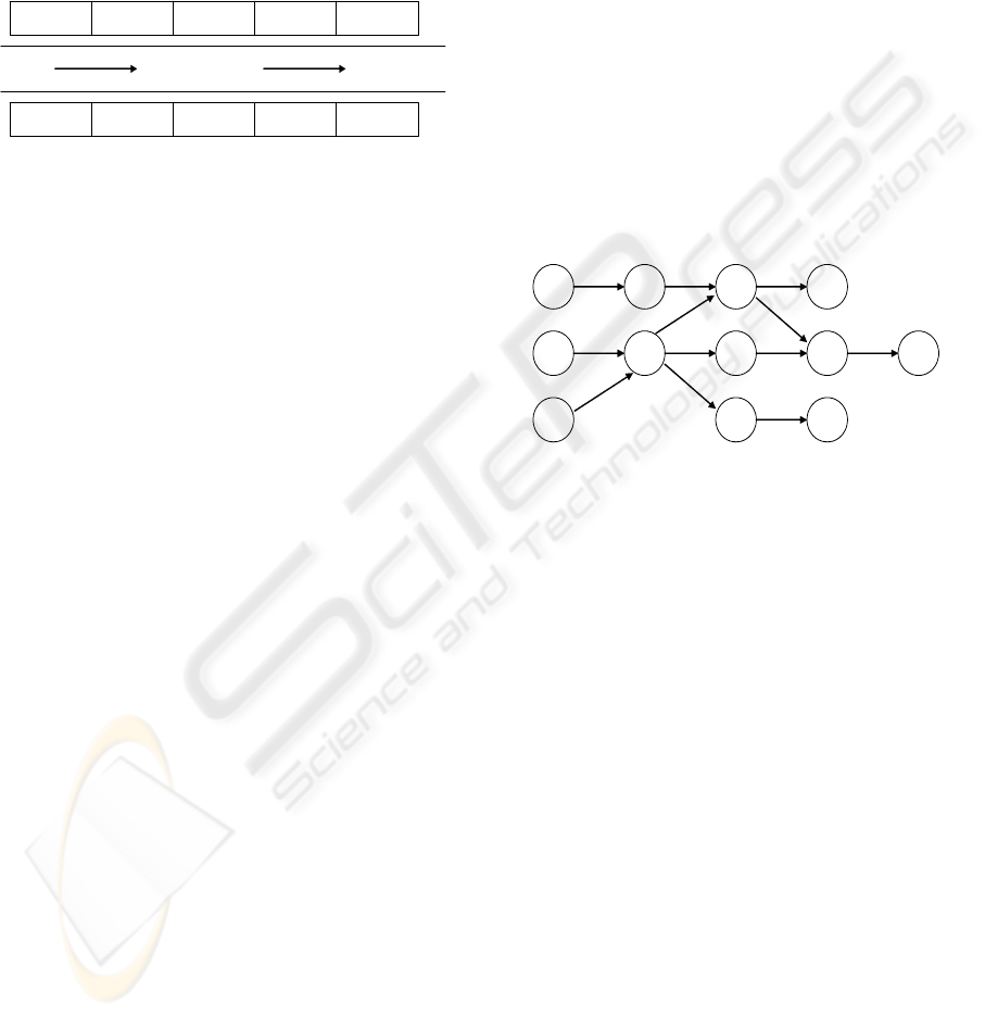
A line balancing problem is usually represented

by a precedence diagram as illustrated in Figure 2. A

circle indicates a task, and an arc linking two tasks

represents the precedence relation between the tasks.

Each task is associated with a label of (t

, d), where t

is the task processing time and d (=L, R or E) is the

preferred operation direction. L and R, respectively,

indicate that the task should be assigned to a left-

and a right-side station. A task associated with E can

be performed at either side of the line.

While balancing assembly lines, it is generally

needed to take account of the features specific to the

lines. In a one-sided assembly line, if precedence

relations are considered appropriately, all the tasks

assigned to a station can be carried out continuously

without any interruption. However, in a two-sided

assembly line, some tasks assigned to a station can

be delayed by the tasks assigned to its companion

(Bartholdi, 1993). In other words, idle time is

sometimes unavoidable even between tasks assigned

to the same station. Consider, for example, task j and

its immediate predecessor i. Suppose that j is

assigned to a station and i to its companion station.

Task j cannot be started until task i is completed.

Therefore, balancing such a two-sided assembly

line, unlike a one-sided assembly line, needs to

consider the sequence-dependent finish time of

tasks.

Figure 2: Precedence graph (cycle time =16).

This notion of sequence dependency further

influences the treatment of cycle time constraint.

Every task assigned to a station must be able to be

completed within a predetermined cycle time. In a

one-sided assembly line, this can readily be achieved

by checking the total operation time of tasks

assigned to a station. Therefore, a task not violating

any precedence constraints can be simply added to

the station if the resulting total amount of operation

time does not exceed the cycle time. However, in a

two-sided assembly line, due to the above sequence-

dependent delay of tasks, the cycle time constraint

should be more carefully examined. The amount of

time required to perform tasks allocated to a station

is determined by the task sequences in both sides of

the mated-station as well as their operation time. It

should be mentioned that two-sided assembly line is

a special case of single assembly line. Therefore it is

possible to use some procedures and measurements,

which were for simple assembly line developed.

(4, L)

(5, E)

(3, R)

(

, L)

(4, E)

(4, R)

(5, L)

(4, E) (5, E)

(8, E)

(

, E)

(1, R)

ICINCO 2008 - International Conference on Informatics in Control, Automation and Robotics

232

3 HEURISTIC APPROACH

3.1 Grouping Tasks

A task group consists of a considered task i and all

of its predecessors. Such groups are generated for

every un–assigned task. As mentioned earlier,

balancing a two–sided assembly line needs to

additionally consider operation directions and

sequence dependency of tasks, while creating new

groups (Kim et. al, 2005).

While forming initial groups IG(i), the operation

direction is being checked all the time. It’s

disallowed for a group to contain tasks with

preferred operation direction from opposite sides.

But, if each task in initial group is E – task, the

group can be allocated to any side. In order to

determine the operation directions for such groups,

the rules (direction rules DR) are applied:

DR 1. Set the operation direction to the side where

tasks can be started earlier.

DR 2. The start time at both sides is the same, set the

operation direction to the side where it’s expected to

carry out a less amount of tasks (total operation time

of unassigned L or R tasks).

Generally, tasks resulting from “repeatability test”

are treated as starting ones. But there is exception in

form of first iteration, where procedure starts from

searching tasks (initial tasks IT), which are the first

ones in precedence relation. After the first step in the

first iteration we get:

IG (1) = {1}, Time{IG (1)} = 2, Side{IG (1)} = ‘L’

IG (2) = {2}, Time{IG (2)} = 5, Side{IG (2)} = ‘E’

IG (3) = {3}, Time{IG (3)} = 3, Side{IG (3)} = ‘R

where:

Time{IG(i)} – total processing time of i

initial

group,

Side{IG(i)} – preference side of i

initial group.

To those who are considered to be the first, the next

tasks will be added, (these ones which fulfil

precedence constraints).

Whenever new tasks are inserted to the group i, the

direction, cycle time and number of immediate

predecessors are checked. If there are more

predecessors than one, the creation of initial group j

comes to the end.

First iteration – second step

IG (1) = {1, 4, 6}, Time{IG (1)} = 8, Side{IG (1)}

= ‘L’

IG (2) = {2, 5}, Time{IG (2)} = 9 , Side{IG (2)} =

‘E’

IG (3) = {3, 5} , Time{IG (3)} = 7 , Side{IG (3)} =

‘R’

When set of initial groups is created, the last

elements from those groups are tested for

repeatability. If last element in set of initial groups

IG will occur more than once (groups pointed by

arrows), the groups are intended to be joined – if

total processing time (summary time of considered

groups) is less or equal to cycle time. Otherwise,

these elements are deleted.

In case of occurring only once, the last member

is being checked if its predecessors are not contained

in Final set FS. If not, it’s removed as well. So far,

FS is empty.

First iteration – third step

IG (1) = {1, 4}, Time{IG (1)} = 4, Side{IG (1)} =

‘L’

IG (2) = {2, 3, 5}, Time{IG (2)} = 12, Side{IG (2)}

= ‘R’

Whenever two or more initial groups are joined

together, or when initial group is connected with

those one coming from Final set – the “double task”

is added to initial tasks needed for the next iteration.

In the end of each iteration, created initial groups are

copied to FS.

First iteration – fourth step

FS = { (1, 4); (2, 3, 5) },

Side{FS (1)} = ‘L’, Side{FS (2)} = ‘R’

Time {FS(2)} = 12, Time {FS(1)} = 14,

IT = {5}.

In the second iteration, second step, we may notice

that predecessor of last task coming from IG(1) is

included in Final Set, FS(2). The situation results in

connecting both groups under holding additional

conditions:

Side{IG(1)} = Side{FS(2)},

Time + time < cycle.

After all, there is no more IT tasks, hence,

preliminary process of creating final set is

terminated.

The presented method for finding task groups is to

be summarized in simplified algorithm form. Let U

denote to be the set of un – assigned tasks yet and

TWO-SIDED ASSEMBLY LINE - Estimation of Final Results

233

be a task group consisting of task i and all its

predecessors (excluded from U set).

STEP 1. If U = empty, go to step 5, otherwise,

assign starting task from U.

STEP 2. Identify IG

. Check if it contains tasks with

both left and right preference operation direction,

then remove task i.

STEP 3. Assign operation direction Side{ IG

} of

group IG

. If IG

has R-task (L-task ), set the

operation direction to right (left). Otherwise, apply

so called direction rules DR.

STEP 4. If the last task i in IG

is completed within

cycle time, the IG

is added to Final set of

candidates FS(i). Otherwise, exclude task i from IG

and go to step 1.

STEP 5. For every task group in FS(i), remove it

from FS if it is contained within another task group

of FS.

The resulting task groups become candidates for the

mated-station.

FS = {(1,4), (2,3,5,8)}.

3.2 Groups Assignment

The candidates are produced by procedures

presented in the previous section, which claim to not

violate precedence, operation direction restrictions,

and what’s more it exerts on groups to be completed

within preliminary determined cycle time. Though,

all of candidates may be assigned equally, the only

one group may be chosen. Which group it will be –

for this purpose the rules helpful in making decision,

will be defined and explained below:

AR 1. Choose the task group FS(i) that may start at

the earliest time.

AR 2. Choose the task group FS(i) that involves the

minimum delay.

AR 3. Choose the task group FS(i) that has the

maximum processing time.

In theory, for better understanding, we will consider

a left and right side of mated – station, with some

tasks already allocated to both sides. In order to

achieve well balanced station, the AR 1 is applied,

cause the unbalanced station is stated as the one

which would probably involve more delay in future

assignment. This is the reason, why minimization

number of stations is not the only goal, there are also

indirect ones, such as reduction of unavoidable

delay. This rule gives higher priority to the station,

where less tasks are allocated. If ties occurs, the AR

2 is executed, which chooses the group with the least

amount of delay among the considered ones. This

rule may also result in tie. The last one, points at

relating work within individual station group by

choosing group of task with highest processing time.

For the third rule the tie situation is impossible to

obtain, because of random selection of tasks. The

implementation of above rules is strict and easy

except the second one. Shortly speaking, second rule

is based on the test, which checks each task

consecutively, coming from candidates group FS(i)

– in order to see if one of its predecessors have

already been allocated to station. If it has, the

difference between starting time of considered task

and finished time of its predecessor allocated to

companion station is calculated. The result should be

positive, otherwise time delay occurs.

3.3 Final Procedures

Having rules for initial grouping and assigning tasks

described in previous sections, we may proceed to

formulate formal procedure of solving two – sided

assembly line balancing problem (Kim et. al, 2005).

Let us denote companion stations as j and j’,

D(i) – the amount of delay,

Time(i) – total processing time (Time{FS(i)}),

S(j) – start time at station j,

STEP 1. Set up j = 1, j’ = j + 1, S(j) = S(j’) = 0, U –

the set of tasks to be assigned.

STEP 2. Start procedure of group creating (3.2),

which identifies

FS = {FS(1), FS(2), …, FS(n)}. If FS = ∅, go to

step 6.

STEP 3. For every FS(i), i = 1,2, … , n – compute

D(i) and Time(i).

STEP 4. Identify one task group FS(i), using AR

rules in Section 3.3

STEP 5. Assign FS(i) to a station j (j’) according to

its operation direction, and update S(j) = S(j) +

Time(i) + D(i). U = U – {FS(i)}, and go to STEP 2.

STEP 6. If U

≠

∅, set j = j’ + 1, j’ = j + 1, S(j) =

S(j’) = 0, and go to STEP 2, Otherwise, stop the

procedure.

4 MEASURES OF FINAL

RESULTS OF ASSEMBLY LINE

BALANCING PROBLEM

Some measures of solution quality have appeared in

line balancing problem. Below are presented three of

them (Scholl, 1998).

Line efficiency (LE) shows the percentage

utilization of the line. It is expressed as ratio of total

station time to the cycle time multiplied by the

number of workstations:

ICINCO 2008 - International Conference on Informatics in Control, Automation and Robotics

234

where:

K - total number of workstations,

c - cycle time.

Smoothness index (SI) describes relative

smoothness for a given assembly line balance.

Perfect balance is indicated by smoothness index 0.

This index is calculated in the following manner:

where:

max

= maximum station time (in most cases

cycle time),

= station time of station i.

Time of the line (LT) describes the period of

time which is need for the product to be completed

on an assembly line

where:

c - cycle time,

K -total number of workstations.

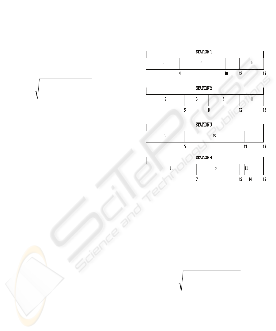
5 NUMERICAL RESULTS

The results of proposed procedure for the example

from Figure 2 are given in a Gantt chart – Figure 3.

Before presenting performance measures for current

example, it would be like to stress difference in

estimation of line time form, resulting from

restrictions of parallel stations. In two – sided line

method within one mated-station, tasks are intended

to perform its operations at the same time, as it is

shown in example in Figure.3, where tasks 7, 11

respectively are processed simultaneously on single

station 3 and 4, in contrary to one – sided heuristic

methods. Hence, modification has to be introduced

to that particular parameter which is the

consequence of parallelism. Having two mated-

stations from Figure 3, the line time LT is not 3*16

+ 13, as it was in original expression. We must treat

those stations as two double ones (mated-stations),

rather than individual ones S

. Accepting this line of

reasoning, new formula is presented below:

where:

Km – number of mated-stations

K – number of assigned single stations

t(S

) – processing time of the last single

station

Figure 3: Results for the example problem.

As far as smoothness index and line efficiency are

concerned, its estimation, on contrary to LT, is

performed without any change to original version.

These criterions simply refer to each individual

station, despite of parallel character of the method.

But for more detailed information about the balance

of right or left side of the assembly line additional

measures will be proposed:

Smoothness index of the left side

where:

- smoothness index of the left side of two-sided

line

maxL

- maximum of duration time of left allocated

stations

- duration time of i-th left allocated station

Smoothness index of the right side

100%

⋅

∑

(1)

()

∑

−=

imax

STSTSI

(2)

()

T1KcLT +−⋅=

(3)

() }{

)t(S),t(SMax1KmcLT

1KK −

+−⋅=

(4)

()

∑

−=

iLmaxLL

STSTSI

(5)

TWO-SIDED ASSEMBLY LINE - Estimation of Final Results

235

where:

- smoothness index of the right side of two-sided

line

maxR

- maximum of duration time of right allocated

stations

- duration time of i-th right allocated station

Table 1: Numerical results.

Name Value

LE 84,38%

LT 30

SI 4,69

The numerical results of different measures in Table

1 are given. The value of line efficiency is

acceptable, smoothness indexes of the right and left

side of the line show which part of the assembly line

is better balanced. The smoothness index SI informs

about balance of the whole line. It is possible to

compare the two-sided line balance with single

assembly line balance and to consider the influence

of position restrictions (L,R or E).

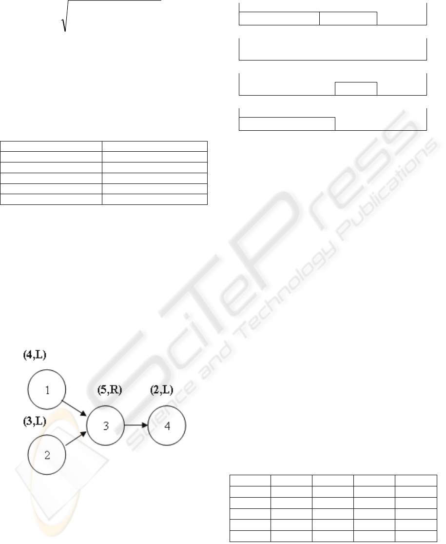
Next it will be consider a small example

presented in Figure 4.

Figure 4: Precedence graph (4 tasks, c=10).

In this point, it’s worth to mention about a special

case, when mated-station includes instead of two

stations, just one. Such a situation takes place, where

one station is loaded to a certain point that not

allows for assigning any more tasks for this part of

the line. As the result, one station stays empty.

Balance of this case is presented in Figure 5.

Figure 5: Balance of two-sided line (N=4, c=10).

In this case we got an assembly line which is a structure of

incomplete two-sided assembly line. It is possible to

estimate the balanced line in two ways: as a single line

with parallel stations or incomplete two-sided line.

In the first case we obtain:

K = 3

LE = 46,67%

SI = 9,9

Considering this case as two-sided line we get:

K = 4

LE = 35%

= 11,18

= 8,54

SI = 14,07

As we can see there are some differences in final

measurements of the balanced line. The reason is

that using heuristic methods we design two-sided

assembly line. These kinds of heuristics are very

sensitive to cycle time value. Some final balances

for different value of cycle time for an example from

Figure 2 in Table 2 are shown.

Table 2: Final results of different measures (c = var).

c K LT SI LE

14 6 37 15,81 66,67%

15 6 39 17,66 62,22%

16 4 30 4,69 84,38%

17 6 43 22,05 54,90%

18 4 32 4,69 77,70%

()

∑

−=

iRmaxRR

STSTSI

(6)

TATI

STATION 2

STATION 3

STATION 4

ICINCO 2008 - International Conference on Informatics in Control, Automation and Robotics

236

6 CONCLUSIONS

Two-sided assembly lines become more popular in

last time. Therefore it is obvious to consider this

structure using different methods. In this paper a

heuristic approach was discussed. Two-sided

assembly line structure is very sensitive to changes

of cycle time values. It is possible very often to get

incomplete structure of the two-sided assembly line

(some stations are missing) in final result. We can

use different measures for comparing the solutions

(line time, line efficiency, smoothness index).

Author proposes additionally two measures:

smoothness index of the left side (SI

) and

smoothness index of the right side (SI

) of the two-

sided assembly line structure. These measurements

allow to get more knowledge about allocation of the

tasks and about the balance on both sides.

This research was supported by grant of Ministry

of Science and Higher Education 3T11Ao2229 in

2005-2008.

REFERENCES

Bartholdi J.J., 1993. Balancing two-sided assembly lines:

a case study, International Journal of Production

Research, 23, 403-421

Baybars, I., 1986. A survey of exact algorithms for simple

assembly line balancing problem, Management

Science, 32, 11-17

Eral, Erdal, Sarin S.C., 1998. A survey of the assembly

line balancing procedures, Production Planning and

Control, 9, 34-42

Forteca D.J., Guest C.L., Elam M., Karr C.L., 2005. A

fuzzy logic approach to assembly line balancing,

Mathare & Soft Computing, 57-74

Gutjahr, A.L., Neumhauser G.L., 1964, An algorithm for

the balancing problem, Management Science, 11, 23-

Halgeson W. B., Birnie D. P., 1961. Assembly line

balancing using the ranked positional weighting

technique, Journal of Industrial Engineering, 12, 18-

Kao, E.P.C., 1976. A preference order dynamic program

for stochastic assembly line balancing, Management

Science, 22, 19-24

Lee, T.O., Kim Y., Kim Y.K., 2005. Two-sided assembly

line balancing to maximize work relatedness and

slackness, Computers & Industrial Engineering, 40,

273-292

Salveson, M.E., 1955. The assembly line balancing

problem, Journal of Industrial Engineering, 62-69

Scholl, A., 1998. Balancing and sequencing of assembly

line, Physica- Verlag

Sury, R.J., 1971. Aspects of assembly line balancing,

International Journal of Production Research, 9, 8-14

TWO-SIDED ASSEMBLY LINE - Estimation of Final Results

237