PARAMETERIZATION AND INITIALIZATION OF BEARING-ONLY

INFORMATION

A Discussion

R. Aragues and C. Sagues

DIIS - I3A, University of Zaragoza, Mar´ıa de Luna, 50018 Zaragoza, Spain

Keywords:

Bearing-only, Feature parameterization: cartesian and inverse-depth, Delayed/Undelayed initialization.

Abstract:

In this paper we discuss feature parameterization and initialization for bearing-only data obtained from vision

sensors. The interest of this work refers to the comparison of the bearing-only data representation and ini-

tialization techniques. The behavior of the algorithm is analyzed for different robot motions and depth of the

features. The results are evaluated in terms of the sensitivity to step size and performance to ill conditioned

situations. The problem studied refers to robots moving on the plane, sensing the environment and extract-

ing bearing-only information from uncalibrated cameras to recover the position of the landmarks and its own

localization.

1 INTRODUCTION

The manipulation of bearing information is an impor-

tant issue in robotics. Bearing-only data is the kind of

information provided by cameras through the projec-

tion of landmarks which are in the scene. In order to

recover the position of these landmarks in the world,

multiple observations taken from different positions

must be combined.

Compared with information extracted from other

sensors such as lasers, bearing information is compli-

cated to use. However, the multiple beneﬁts of using

cameras havemotivated the interest in the researchers.

These beneﬁts include the property that cameras are

able to sense quite distant features so that the sensing

is not restricted to a limited range.

This sensing of the environment in the form of

bearing information may be used for many applica-

tions such as the computation of the landmark local-

ization in the environment or the calculation of the

own robot pose mostly known as SLAM Simultane-

ous Localization and Mapping.

Algorithms which use bearing information must

deal with the problem of creating representations for

features by the combination of bearing data. The

problem of feature parameterization and feature ini-

tialization are of big importance here.

With regard to the feature parameterization, the

classical approach has been the use of a cartesian

parameterization (Bailey, 2003), (Kwok and Dis-

sanayake, 2004), (Costa et al., 2004), (Klippenstein

et al., 2007). Some approaches prefer a depth param-

eterization, where features are stored as an starting

point of the ray where the feature lays, the inclina-

tion of the ray and the depth (Davison, 2003). An

inverse-depth parameterization is an alternative, simi-

lar to the depth parameterization but using the inverse

of the depth instead (Montiel et al., 2006). Some ap-

proaches use no explicit feature parameterization and

instead represent landmarks as constraints between

three robot poses (Trawny and Roumeliotis, 2006).

With regard to the feature initialization, Unde-

layed techniques immediately introduce features in

the map so that they can be used to improve the

robot estimation (Montiel et al., 2006), (Trawny and

Roumeliotis, 2006), (Costa et al., 2004), (Kwok and

Dissanayake, 2004) while Delayed techniques defer

the introduction into the map until the features are

near-Gaussian (Bailey, 2003), (Klippenstein et al.,

2007). Delayed techniques often create temporal rep-

resentations for landmarks which are maintained in

separate ﬁlters and evolve with the incorporation of

new observations of these landmarks until they are ﬁ-

nally introduced into the map (Davison, 2003).

The problem of depth computation for landmarks

is afforded in two separate ways. Some approaches

create depth representation from only one bearing as-

suming an approximate value for it. These techniques

are able to cover depths from the position were the

landmark was observed until inﬁnity or until a max-

252

Aragues R. and Sagues C. (2008).

PARAMETERIZATION AND INITIALIZATION OF BEARING-ONLY INFORMATION - A Discussion.

In Proceedings of the Fifth International Conference on Informatics in Control, Automation and Robotics - RA, pages 252-261

DOI: 10.5220/0001500002520261

 SciTePress

imum depth within the workspace (Kwok and Dis-

sanayake, 2004), (Davison, 2003), (Montiel et al.,

2006). The other approach to depth computation is

the combination of observations taken from differ-

ent robot poses, where triangulation techniques are

used to recover the depth (Bailey, 2003), (Klippen-

stein et al., 2007).

The interest of this work refers to the comparison

of the bearing-only data representations and initial-

ization techniques, analyzed for different robot mo-

tions relative to depth of the landmarks in the scene.

Two feature parameterizations are studied. The ﬁrst

is an standard cartesian parameterization, where fea-

tures are described by their (x,y) position. The alter-

native representation is an adaptation of the inverse-

depth (Montiel et al., 2006) to the 2D situation. Be-

sides, both Undelayed and Delayed strategies for fea-

ture initialization are used and their performance is

compared in different scenarios.

The problem studied in this paper refers to robots

moving on the plane, sensing the environment and ex-

tracting bearing-only information from uncalibrated

images to recover the position of the landmarks and

its own localization. As a result of this investigation,

some theoretical solutions are proposed, and their va-

lidity is supported by an exhaustive experimentation

using simulated data. Some preliminary experiments

have been carried out using real data from omnidirec-

tional images.

2 BACKGROUND

The problem studied in this paper is related to the use

of bearing-only information for the SLAM problem

using EKF. The robot moves on the plane and ele-

ments in the map are represented by their 2D coor-

dinates. Robot observes landmarks within a ﬁeld of

view of 360

◦

due to the use of omnidirectional cam-

eras and obtains bearing-only measurements. Odom-

etry is used to predict robot motion in every step. The

EKF Extended Kalman Filter is a widely used tech-

nique in these problems and a lot of information can

be found in the literature. The data association prob-

lem is not discussed in this paper. An innovation test

is used to select the observations which will be used

in the ﬁlter update. This test computes an individ-

ual compatibility for all observation-prediction pairs

and then obtains the greatest set of jointly compatible

pairs using the JCBB algorithm (Neira and Tard´os,

2001). Although traditionally this algorithm is used

to solve the data association problem, we use it in or-

der to avoid the ﬁlter divergence in the presence of

poorly initialized features or high innovations.

Along this paper, next notation will be used:

x = (x

...x

): the state vector containing cur-

rent robot pose (x

) and the positions of landmarks

...x

)

P: the covariance matrix.

= (x

,θ

) ∈ R

, θ

⊂ [−π,π] , for j =

1..k: j-th robot pose. When there is no confusion, the

subscript j is omitted.

= (x

) ∈ R

, for i = 1..n: Position of the i-

th feature in the map, for cartesian parameterization,

or x

= (x

,θ

,ρ

) ∈ R

, θ

⊂ [−π,π], for i = 1..n:

when referring to inverse-depth parameterization.

: measurement taken from robot pose j to fea-

ture i. When only one robot pose is used, z

refers to

the observation of feature i.

3 FEATURE

PARAMETERIZATION

Cartesian parameterizations represent features by

their (x,y) coordinates. This parameterization is very

intuitive since the feature position within the map can

be easily obtained. The initialization of features in

this cartesian parameterization is problematic due to

the nonlinearity of the triangulation techniques used

to recover its position based on the observations taken

from different robots poses. It can be easily shown

that bearings generate bigger uncertainty as landmark

position goes away from the camera. The observation

model for a feature x

= (x

) observed from a robot

pose x

= (x

,θ

) is (Bailey, 2003):

= h(x

) = arctan



− y

− x



− θ

(1)

Inverse-depth parameterizations represent a fea-

ture x

as a ray starting at (x

), the position where

the feature was ﬁrstly observed, with a global bearing

and a depth of

. Every feature is stored in the

state vector using these four parameters (x

,θ

,ρ

The cartesian coordinates of the landmark could be

calculated as:





(2)

where m

= [cos(θ

)sin(θ

)]

The observation model with inverse-depth for a

feature x

= (x

,θ

,ρ

) observed from a robot pose

= (x

,θ

) is:

h = atan2(h

) (3)

PARAMETERIZATION AND INITIALIZATION OF BEARING-ONLY INFORMATION - A Discussion

253

where (h

) are the coordinates of the feature in

the robot reference:





= R





−





(4)

with R



cosθ

sinθ

−sinθ

cosθ



This observation model remains valid if next

equation is used instead of equation 4 provided that

> 0:





= R







−





+ m



(5)

As advantage with respect to the cartesian pa-

rameterization, the observation model for the inverse

depth is near linear. Additionally, landmarks at in-

ﬁnity (ρ

= 0) or uncertainties that extend to inﬁn-

ity can be represented. The main drawback of the

inverse-depth is that features are over-parameterized,

and therefore the Covariance matrix size is greater.

4 FEATURE INITIALIZATION

The feature initialization in SLAM consists in the cre-

ation of a representation of the landmark’s position

and its introduction into the stochastic map through

its mean and its covariance matrix. The feature ini-

tialization problem of bearing-only is due to the fact

that features are only partially observable.

As told, a measurement only gives information

about the direction towards the landmark and two or

more observations must be combined in order to re-

cover the depth of the landmark. However, there are

some situations where the depth cannot be recovered

Next we give a formal description of these situations.

Theorem 1.- Let us name x

a robot position and x

second position translated but not rotated with respect

to x

. Let us name z

the observation of a feature x

taken from x

and z

the observation of the same

feature taken from x

. Let us name d

the transla-

tion from x

to x

on a perpendicular direction to

and d

the translation on a parallel direction to z

Without loss of generality, let d

be equal to zero. The

landmark depth (distance between x

and the land-

mark) can be totally determined from α = z

− z

depth = d

/tanα (6)

Corollary 1.1.- This is an undetermined problem

(0/0) when simultaneously d

= 0 and α = 0 + kπ

for k ∈ Z.

Corollary 1.2.- This problem remains undetermined

independently of the magnitude of d

Corollary 1.3.- The landmark is at inﬁnity if simulta-

neously α = 0 + kπ for k ∈ Z and d

is different of

zero .

Theorem 2.- Let us name x

a robot position and x

second position rotated but not translated with respect

to x

. Let us name z

the observation of a feature x

taken from x

and z

the observation of the same

feature taken from x

. Robot rotation (θ

) can be

absolutely determined from θ

= z

− z

Corollary 2.1.- Given a pure rotation motion, feature

depth cannot be recovered.

Corollary 2.2.- Given a translation and rotation mo-

tion with landmarks of inﬁnite depth, the robot rota-

tion can be computed from z

− z

for any d

< ∞

and robot translation cannot be recovered.

Based on these theorems, ill-conditioned situa-

tions are identiﬁed:

Proposition 1.- Depth of features aligned with robot

trajectory cannot be recovered. This situations is for-

malized in Corollaries 1.1 and 1.2.

Proposition 2.- Depth cannot be recovered with pure

rotation motions as shown in Corollary 2.1.

Proposition 3.- Landmarks at inﬁnity give robot ori-

entation, but no translation information can be ob-

tained from them.This is based on Corollary 2.2.

Feature estimates calculated when the depth com-

putation problem is ill-conditioned present high co-

variances and great estimation errors which may

cause linealization problems. Once a feature has been

wrongly initialized, new observations taken from

robot poses not aligned with the feature will not be

able to correct its position. If a cartesian parameter-

ization is used, an additional problem is that features

with inﬁnite depth cannot be represented and their ini-

tialization must be deferred. This situation is formal-

ized in Corollary 1.3.

4.1 Undelayed Initialization

The undelayed initialization consists in the introduc-

tion of landmarks into the system the ﬁrst time the

landmark is observed. This technique presents many

beneﬁts since the information attached to a landmark

can be used earlier and it allows the use of landmarks

which may never been initialized if a delayed strat-

egy is used.Since the ﬁrst time a landmark is observed

only bearing information is available, undelayed tech-

niques must deal with the problem of creating a repre-

sentation for the depth and its associated uncertainty.

If an inverse-depth parameterization is used, land-

marks are introduced using a ﬁxed initial depth and an

uncertainty representation is created which covers all

ICINCO 2008 - International Conference on Informatics in Control, Automation and Robotics

254

depths from some d

min

to inﬁnity. This initial depth

must be adjusted depending on the workspace.

Since cartesian parameterization requires low co-

variances, an undelayed initialization is only possible

if multiple hypothesis in depth are created (Kwok and

Dissanayake, 2004), (Kwok et al., 2007), (Sola et al.,

2005). All these approaches present a high complex-

ity and size of the map. Due to this complexity, ap-

proaches using undelayed initialization together with

cartesian parameterization are no longer analyzed in

this paper.

4.2 Delayed with Two Observations

This delayed technique consists in the combination of

the ﬁrst two observations of a landmark to recover its

position using a triangulation algorithm. This is a not

purely delayed technique, since there are no condi-

tions which must be satisﬁed by the observations in

order for the landmark to be initialized, and all land-

marks are introduced in the map provided that they

are observed from at least two robots poses. The main

beneﬁt of this initialization strategy is that the solution

is independent on the workspace. However, triangula-

tion algorithms used to recover the landmark position

are highly non-linear and, depending on the arrange-

ment of robot poses and features, the problem may be

ill-conditioned.

If a cartesian parameterization is used, the recov-

ered feature position must be near-Gaussian and co-

variances must be small. For this reason, additional

tests are used to check that features satisfy these con-

ditions. If features are parameterized using inverse-

depth, this strategy may suppose a beneﬁt in the sense

that it is independent on the size of the scene. There-

fore higher covariances in the estimates are admissi-

ble and recovered features are near-Gaussian even for

low parallaxes.

4.3 Delayed until Condition

In a pure delayed initialization technique, observa-

tions of landmarks are accumulated and its initializa-

tion is deferred until a condition of Gaussianity is sat-

isﬁed; then observations are used to create a repre-

sentation for the feature (Bailey, 2003), (Klippenstein

et al., 2007).

If a delayed initialization is used, some landmarks

may neverbeen initialized. Since the information pro-

vided by landmarks cannot been used until the land-

mark is initialized, a delayed technique decreases the

amount of information available to improve robot the

pose. Many delayed techniques present a high com-

putational cost to calculate the condition, and have

their own problems and limitations. The main beneﬁt

is that the representation for the landmark is more ac-

curate and reliable than the obtained by an undelayed

strategy.

5 DISCUSSION

As told, the aim of this work is the comparison of

cartesian and inverse-depth parameterizations com-

bined with delayed and undelayed initialization tech-

niques. These have been selected because are the

most commonly used, being also simple and of low

computational complexity.

5.1 Inverse-Depth Undelayed

This technique is an adaptation to the 2D situation of

the technique described in (Montiel et al., 2006). A

feature x

is introduced into the map using a single

observation. The current robot pose x

= (x

,θ

)

is used together with the observation z

and an ini-

tial depth ρ

parameterized in inverse-depth to get the

feature representation x

. This depth is worked out

using a minimal distance d

min

which must be selected

depending on the workspace:

min

;ρ

min

;σ

min

(7)

where ρ

min

is the inverse of depth, ρ

is the ini-

tial inverse-depth, which is the middle value of the

interval [0,ρ

min

], and σ

is the standard deviation

used to initialize ρ

(95% of ρ is in the interval



− 2σ

,ρ

+ 2σ



= [0, ρ

min

].) The initial value of

the feature is calculated as:

= g(x

,ρ

) = (x

,θ

+ z

,ρ

) (8)

5.2 Inverse-Depth Delayed with Two

Observations

As a proposal, an inverse-depth parameterization

(Montiel et al., 2006) is combined with a delayed ini-

tialization technique where the second observation is

used to calculate the initial depth for the feature. The

position for the feature x

which has been observed

from x

and x

producing measurements z

and z

is calculated as follows:

= g(x

) = (x

,θ

+ z

,ρ

)

∗c

−c

∗s

−y

)∗c

−(x

−x

)∗s

(9)

PARAMETERIZATION AND INITIALIZATION OF BEARING-ONLY INFORMATION - A Discussion

255

where c

= cos(θ

+ z

) and s

= sin(θ

+ z

), for

j = 1,2.

An additional test is used in order to detect situ-

ations where inverse-depth cannot be recovered and

intersections take place in the opposite direction of

the observation. In these situations, the initialization

is deferred.

5.3 Cartesian Delayed with Two

Observations

Given the ﬁrst two observations z

of a landmark

taken from robot poses x

, the landmark po-

sition x

= (x

) is calculated as follows (Bailey,

2003):

= g

) =

−x

−(y

−y

−s

= g

) =

−y

+(x

−x

−s

(10)

where c

= cos(θ

+ z

) and s

= sin(θ

+ z

), for

j = 1,2.

Similarly a test is used to check that features can

be recovered and intersections of bearings are not in

the opposite direction of the observations.

5.4 Cartesian/Inverse-Depth Delayed

until Finite Depth

A delayed technique is proposed where feature ini-

tialization is deferred until ﬁnite uncertainty in depth

can be estimated.

This is achieved by a simple test which compares

two observation rays and checks if they are parallel.

This situation is characterized by Corollaries 1.1 and

1.3. When observation rays are parallel, the uncer-

tainty in depth of the recovered landmark extends to

inﬁnity and the initialization is deferred. This test is

especially useful when a cartesian parameterization

is used, since inﬁnite depths cannot been modeled.

Let x

= (x

,θ

), for j = 1, 2 be the two

robot poses where observations z

, for j = 1,2 to

a landmark x

were taken. Global bearings α

, for

j = 1,2 to the landmark are calculated as:

= θ

+ z

(11)

If we name S

the linearized propagated covari-

ance for bearing α

then the Chi-squared test for Fi-

nite Depth is expressed as:

(α

− α

)

α1i

+ S

> χ

0.99,1d.o. f

(12)

5.5 Cartesian/Inverse-Depth Delayed

until Feature Not Aligned with

Robot Poses

As stated in Proposition 1, the initialization of fea-

tures aligned with the robot trajectory is problematic

when working with bearing-only data. When a fea-

ture is observed from two robot poses which are in

line with the feature, it is not possible to make a right

depth initialization. Corollary 1.1. gives a formal

explanation of this situation: feature is aligned with

robot trajectory when the observation rays are paral-

lel and the robot translation takes place in a direction

which is parallel to the observation.

Let x

= (x

,θ

), for j = 1, 2 be the two

robot poses where observations to a landmark x

were

taken. From here α

, α

, for j = 1,2 can be com-

puted with equation 11. Let S

, for j = 1,2 be their

linearized propagated covariances. Observation rays

are parallel when:

(α

− α

)

α1i

+ S

≤ χ

0.99,1d.o. f

(13)

The robot trajectory from x

to x

has a global

inclination which can be calculated as:

= arctan



− y

− x



(14)

Let S

be the linearized propagatedcovariancefor

bearing θ

. The trajectory is parallel to the observa-

tion rays when:

(θ

− α

)

θt

+ S

≤ χ

0.99,1d.o. f

(15)

for j = 1,2.

The initialization of features is deferred until a

pair of observations is available where the feature is

not aligned with the trajectory. This delayed tech-

nique is less restrictive than the explained in section

5.4 and is specially useful for an inverse-depth param-

eterization since it allows the initialization and the use

of features of inﬁnite depth.

6 EXPERIMENTS

In order to analyze the performance of the different

parameterizations and initialization techniques, some

experiments have been designed so that the perfor-

mance and robustness of the algorithms can be ana-

lyzed.

ICINCO 2008 - International Conference on Informatics in Control, Automation and Robotics

256

The experimentation and analysis of results is car-

ried out using a simulator which presents many ben-

eﬁts. First of all, exactly the same experiment can

be solved by several algorithms so that results are

fully comparable. Besides, ground truth information

is available to compare with the obtained results.

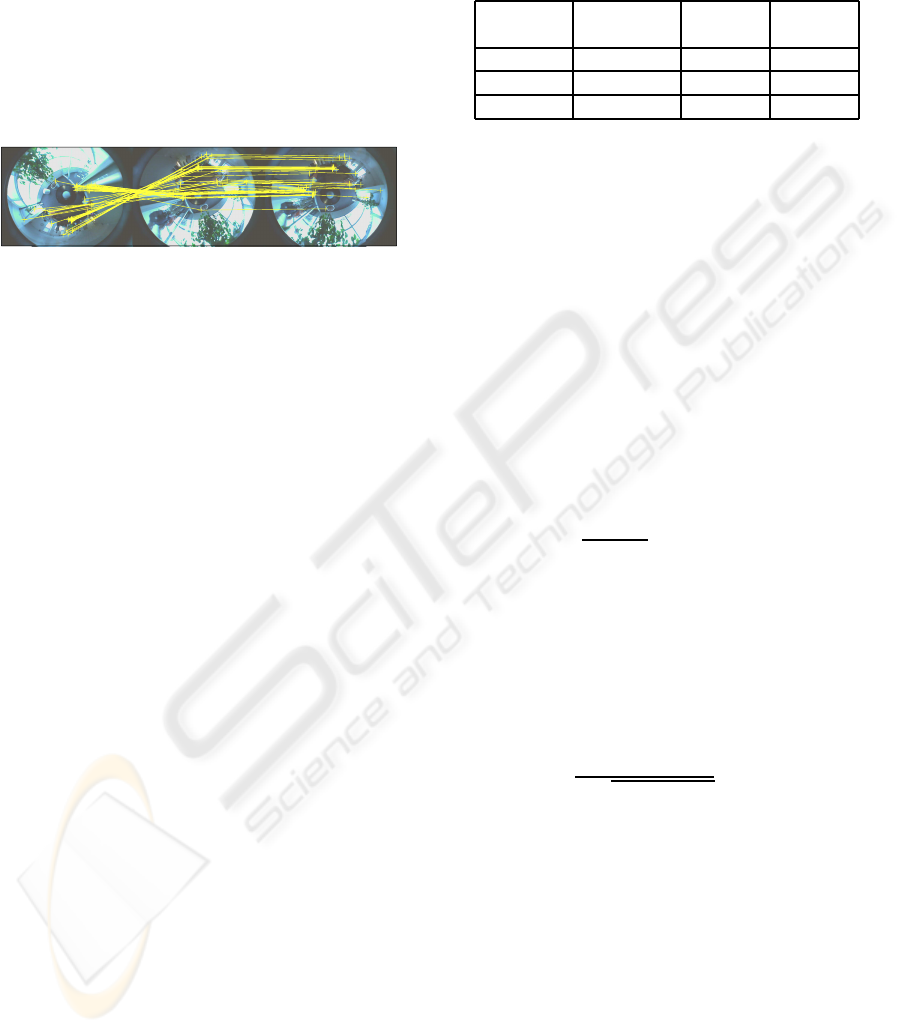
Some preliminary experiments have been carried

out using omnidirectional images which can be seen

in Figure 1. The matches have been obtained using

SURF descriptors (Murillo et al., 2007).

Figure 1: Omnidirectional image: feature extraction and

matching.

In the simulated experiments, an observationnoise

with an standard deviation of 0.125 degrees is used.

Features are placed on the walls of a squared room.

An initialization to the system is introduced from

three robot poses and the ﬁrst 5 observed landmarks.

It is based on SFM techniques with the Trifocal Ten-

sor (Sag¨u´es et al., 2006). The data association prob-

lem is not discussed in this paper and data association

is supposed to be perfect.

Algorithms have been tested in different scenarios

and under different conditions of visibility, trajectory

and step sizes. The Visibility affects to the number

of visible landmarks. Two possibilities are evaluated:

Total, where all features are visible from all robot

poses and Section, where the workspace is divided

into four sections; In every step robot observes the

features within its section and a few from the neigh-

borhood in order to connect the sections. When the

visibility is Total, no loop closing takes place and dis-

tant features are used.

As stated in section 4 the Robot Trajectory has

a big inﬂuence on depth computation in such a way

that if landmark is on the direction of robot transla-

tion, depth computation is an undetermined problem.

Two trajectories have been evaluated. The ﬁrst is an

Squared trajectory composed by several pure trans-

lation motions and four 90

◦

pure rotations. In this

trajectory some features are aligned with the robot

movement for many steps. The odometry noise is in-

troduced as a function of the step size (st) and it can

be seen in columns Pure translation and Pure rotation

of Table 1. The second trajectory is Circular: Robot

describes a circumference when moving along the en-

vironment which supposes mixed rotations and trans-

lations. No feature in the map is observed in line with

the trajectory. The standard deviations of the odome-

try noise are shown in column Mixed motion of Table

Table 1: Odometry noise relative to the step size (st).

Standard Pure Pure Mixed

deviation translation rotation motion

0.01∗ st 0.03∗ st 0.03∗ st

◦

2.5

◦

2.5

◦

The Step Size determines the distance (in meters)

between two consecutive robot poses. This is the pa-

rameter which affects the most the behavior of algo-

rithms. Step sizes of 0.125 m, 0.250 m, 0.5 m and 1

m are tested.

6.1 Analyzed Information

The variables used in order to analyze the perfor-

mance of an algorithm are listed below.

Final Divergence. Percent of results where the ﬁnal

robot pose diverges from its estimation. The condi-

tion which is tested for each component (x

,θ

) in-

dependently can be written as

(a− ba)

> χ

0.99,1d.o. f.

(16)

a being (x

,θ

) the ground-truth, ba the estimated

value for variable a and P its estimated covariance.

Map Consistency. Percent of features in the ﬁnal

map whose estimation is consistent with the ground

truth. A feature is considered consistent if the estima-

tion error in its x

or y

coordinate satisfy:

|a− ba|

P χ

0.99,1d.o. f.

≤ 1.5 (17)

where the variable a represents the x

or y

coordi-

nates.

Trajectory Divergence. Percent of steps in the

trajectory where the estimation of the robot pose (x

, θ

) diverges.

Feature Initialization Step. Average of the number

of steps needed to initialize a feature, calculated as

the difference between the step when a feature is ﬁrst

observed and the one when the feature is introduced

into the map.

Feature Usage. Average of the feature used per step

calculated as the percentage of features used in the

PARAMETERIZATION AND INITIALIZATION OF BEARING-ONLY INFORMATION - A Discussion

257

0.1250.25 0.5 1

100

Final divergence

step size

% final divergence

xy−d

xy−f

xy−l

0.1250.25 0.5 1

100

Map consistency

step size

% consistent features

xy−d

xy−f

xy−l

0.1250.25 0.5 1

100

Trajectory divergence

step size

% steps divergence

xy−d

xy−f

xy−l

(a) (b) (c)

0.1250.25 0.5 1

1.5

2.5

3.5

Feature initialization step

step size

number of steps to initialize features

xy−d

xy−f

xy−l

0.1250.25 0.5 1

100

Feature usage

step size

% features used per step

xy−d

xy−f

xy−l

0.1250.25 0.5 1

100

Map consistency per step

step size

% consistent features per step

xy−d

xy−f

xy−l

(d) (e) (f)

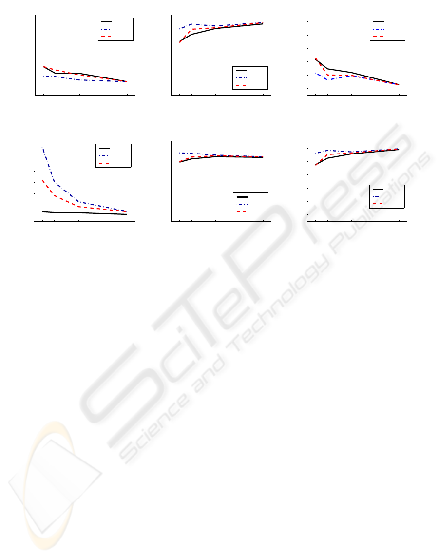
Figure 2: Cartesian delayed techniques comparison. Analysis of the results for different step sizes (x-axis). The algorithms

used are cartesian delayed. xy-d: with two observations. xy-f: until ﬁnite depth. xy-l: until feature not aligned with robot

poses.

ﬁlter update versus the features observed.

Map Consistency per Step. Average of the percent

of consistent features in the map in every step.

Additionally, information related to the precision

and error of the ﬁnal robot pose, the trajectory and the

ﬁnal map has been also studied.

6.2 Results

A total of 160 experiments have been designed, and

all of them have been solved using the available algo-

rithms discussed in section 5. For the Inverse-depth

undelayed, a minimal depth d

min

= 0.5m is used.

The results are analyzed in three different blocks.

In the ﬁrst we compare the cartesian delayed algo-

rithms. In the second, we compare all inverse-depth

delayed approaches and in the third block, a global

comparison is carried out where the best of the carte-

sian delayed algorithms and the inverse-depth de-

layed algorithms are compared to the inverse-depth

undelayed algorithm.

6.2.1 Cartesian Delayed Comparison

The results obtained by the cartesian delayed algo-

rithms can be found in Figure 2. The cartesian de-

layed until ﬁnite depth (xy-f) algorithm performs bet-

ter than the delayed with two observations (xy-d) and

the delayed until features not aligned (xy-l) methods:

the ﬁnal divergence (Figure 2.a) and trajectory diver-

gence (Figure 2.c) are the lowest for all step sizes, the

map consistency (Figure 2.b, Figure 2.f) are the high-

est, and the number of features used to update (Figure

2.e) is higher than the used by the other cartesian al-

gorithms for all step sizes even though this algorithm

needs more steps to initialize a feature (Figure 2.d).

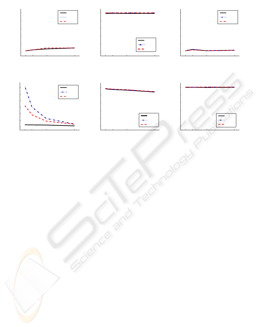
6.2.2 Inverse-depth Delayed Comparison

From the study of the results obtained by the inverse-

depth delayed algorithms, we can observe that all al-

gorithms performed in a very similar way (Figure 3).

The ﬁnal divergence (Figure 3.a), map consistency

(Figure 3.b), trajectory divergence (Figure 3.c), fea-

ture usage (Figure 3.e) and map consistency per step

(Figure 3.f) results are similar for all inverse-depth de-

layed algorithms.Only the feature initialization step

(Figure 3.d) differs, due to the use of the different de-

layed strategies.

An especial study is carried out in order to com-

pare the capability of the inverse-depth algorithms to

deal with features which are observed during many

steps aligned with the trajectory. The most critical sit-

uation is when the robot moves following an squared

trajectory and only observes landmarks within its sec-

ICINCO 2008 - International Conference on Informatics in Control, Automation and Robotics

258

0.1250.25 0.5 1

100

Final divergence

step size

% final divergence

id−d

id−f

id−l

0.1250.25 0.5 1

100

Map consistency

step size

% consistent features

id−d

id−f

id−l

0.1250.25 0.5 1

100

Trajectory divergence

step size

% steps divergence

id−d

id−f

id−l

(a) (b) (c)

0.1250.25 0.5 1

1.5

2.5

3.5

Feature initialization step

step size

number of steps to initialize features

id−d

id−f

id−l

0.1250.25 0.5 1

100

Feature usage

step size

% features used per step

id−d

id−f

id−l

0.1250.25 0.5 1

100

Map consistency per step

step size

% consistent features per step

id−d

id−f

id−l

(d) (e) (f)

Figure 3: Inverse-depth delayed comparison. Analysis of the results for different step sizes (x-axis). The algorithms are: id-d:

with two observations. id-f: until ﬁnite depth. id-l: until feature not aligned with robot poses.

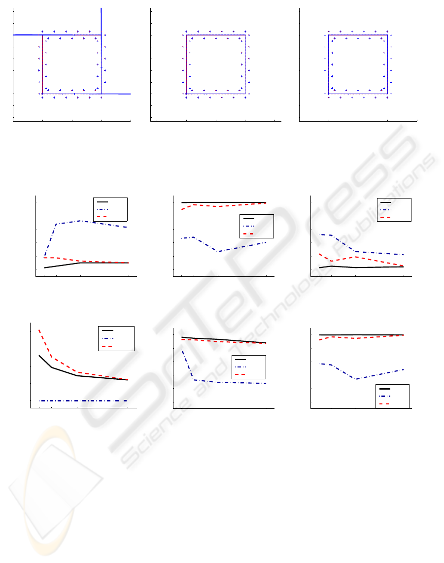
tion. In this situation the problematic features are F12,

F23, and F34 (Figure 4). In this ﬁgure, the ground-

truth robot trajectory and landmark positions are dis-

played in red, while the estimates and uncertainties

calculated by the algorithms are drawn in blue. As

can be observed, both the trajectory and the landmark

positions have been correctly estimated in all cases.

However, features F12, F23 and F34 present high un-

certainty (Figure 4.a) when the algorithm used is the

inverse-depth with two observations (id-d).

Paying attention to the problematic features (F12,

F23, F34) in Figure 4 we can observe the results of

an earlier initialization of features which are in line

with the trajectory. Even though their initial estimate

and covariance correctly represent the feature posi-

tion, posterior observations are not able to correct its

position due to the huge innovation.

The Inverse-depth delayed until ﬁnite depth (id-

f) and Inverse-depth delayed until feature not aligned

with robot poses (id-l) performed in a similar way.

However, the second is preferred because of its capa-

bility to initialize and use features of inﬁnite depth.

6.2.3 Global Comparison

As can be observed in Figure 5, the behavior of the

inverse-depth undelayed algorithm (id-u) is seriously

affected by the step size. For the smallest step size

(0.125m), almost all experimentsconvergedin the last

robot pose (Figure 5.a) while for the other step sizes,

many experiments diverged. The number of consis-

tent features in the ﬁnal map (Figure 5.b) is lower than

for the other algorithms. This behavior is also ob-

served for the number of consistent features per step

(Figure 5.f).

The cartesian delayed until ﬁnite depth algorithm

(xy-f), its behavior is not so much affected by the step

size but we can observe a better performance when

the step size increases: the ﬁnal divergence (Figure

5.a) is slightly higher for smaller step sizes. The num-

ber of consistent features in the ﬁnal map (Figure 5.b)

and along the steps (Figure 5.f) slightly decreases for

smaller step sizes. The feature usage (Figure 5.e) re-

mains high for all step sizes.

The inverse-depth delayed until features not aligned

algorithm (id-l) produced the best results, exhibiting

an stable behavior for all step sizes: almost all ex-

periments converged (Figure 5.a) and also along the

trajectory (Figure 5.c). Almost all features are consis-

tent in the ﬁnal map (Figure 5.b) and along the steps

(Figure 5.f), and the feature usage is the highest (Fig-

ure 5.e).

An interesting information about the features us-

age can be extracted from Figure 5.d and Figure 5.e:

it can be observed that when an undelayed strategy

is selected, the percent of features used to update the

map in every step (Figure 5.e) is much lower than the

PARAMETERIZATION AND INITIALIZATION OF BEARING-ONLY INFORMATION - A Discussion

259

−5 0 5 10 15

−4

−2

F1 F2

F38

F39

F44

F3 F4

F8 F9 F10

F36

F37

F42

F43

F11

F13

F14

F15

F18

F19

F20

F21

F12

F16

F17

F22

F24

F25

F29

F30F31

F23

F26F27F28

F32

F33

F35

F40

F41

F34

FINAL MAP: INVERSE−DEPTH Delayed (two observations)

−5 0 5 10 15

−4

−2

F1 F2

F38

F39

F44

F3 F4

F8 F9 F10

F36

F37

F42

F43

F11

F13

F14

F15

F18

F19

F20

F21

F12

F16

F17

F22

F24

F25

F29F30F31

F23F26F27F28

F32

F33

F35

F40

F41

F34

FINAL MAP: INVERSE−DEPTH Delayed (features not aligned)

−5 0 5 10 15

−4

−2

F1 F2

F38

F39

F44

F36

F37

F42

F43

F9 F10

F14

F15

F18

F19

F20

F21

F11

F13

F12

F16

F22

F25

F30F31

F24

F29

F17

F23F26

F32

F27

F35

F41

F28

F40

F33

F34

FINAL MAP: INVERSE−DEPTH Delayed (Finite depth)

(a) (b) (c)

Figure 4: (a) Inverse-depth delayed with two observations. (b) Inverse-depth delayed until feature not aligned with robot

poses. (c) Inverse-depth delayed until ﬁnite depth.

0.1250.25 0.5 1

100

Final divergence

step size

% final divergence

id−l

id−u

xy−f

0.1250.25 0.5 1

100

Map consistency

step size

% consistent features

id−l

id−u

xy−f

0.1250.25 0.5 1

100

Trajectory divergence

step size

% steps divergence

id−l

id−u

xy−f

(a) (b) (c)

0.1250.25 0.5 1

Feature initialization step

step size

number of steps to initialize features

id−l

id−u

xy−f

0.1250.25 0.5 1

100

Feature usage

step size

% features used per step

id−l

id−u

xy−f

0.1250.25 0.5 1

100

Map consistency per step

step size

% consistent features per step

id−l

id−u

xy−f

(d) (e) (f)

Figure 5: Global comparison. Analysis of the results for different step sizes (x-axis). The algorithms used are: id-u: inverse

depth undelayed, d

min

= 0.5m. xy-f: cartesian delayed until ﬁnite depth. id-l: inverse depth delayed until feature not aligned

with robot poses.

used by the delayed algorithms even though features

initialization requires a lower number of steps (Figure

5.d.) Therefore, delayed techniques provide impor-

tant beneﬁts due to the fact that the initial estimates

introduced into the map are better with lower covari-

ance.

7 CONCLUSIONS

In this paper we have discussed feature parameteri-

zation and initialization using bearing-only measure-

ments. Both considerably affect the results of the al-

gorithms. However, this paper shows that even with

a perfect feature parameterization, if the initialization

problem is ill-conditioned the results are inconsistent.

As conclusion we can state that in general situations

the delayed inverse depth until features not aligned

performs competitively.

An interesting result of this study is the related

ICINCO 2008 - International Conference on Informatics in Control, Automation and Robotics

260

to the cartesian parameterization when it is combined

with a ﬁnite depth test. It was expected that carte-

sian algorithm based in triangulation techniques were

to suffer a great degradation of their performance for

small step sizes. However, results show that the algo-

rithm delayed until ﬁnite depth with cartesian param-

eterization is not very sensitive to the step size and

exhibits very competitive results, which makes it an

appropriate algorithm for indoors. Other interesting

conclusion is that introducing features earlier in the

EKF does not mean that more/better information will

be available to update the state.

In this paper we have also stated ill-conditioned

situations: a pure rotation motion and features aligned

with the trajectory. None of them can be managed in

any case. Some ideas have been presented to detect

these situations which will allow the algorithms to de-

cide which data can be used in each step.

ACKNOWLEDGEMENTS

This work was supported by projects MEC DPI2006-

07928 and IST-1-045062-URUS-STP.

REFERENCES

Bailey, T. (2003). Constrained initialisation for bearing-

only slam. In Proc. IEEE Intl. Conf. on Robotics and

Automation, pages 1996–1971, Taipei, Taiwan.

Costa, A., Kantor, G., and Choset, H. (2004). Bearing-

only landmark initialization with unknown data asso-

ciation. In Proc. of the IEEE Int. Conf. on Robotics

and Automation, pages 1164–1770.

Davison, A. (2003). Real-time simultaneous localisation

and mapping with a single camera. In Proc. Ninth

IEEE Intl.Conf. on Computer Vision.

Klippenstein, J., Zhang, H., and Wang, X. (2007). Feature

initialization for bearing-only visual slam using trian-

gulation and the unscented transform. In Proc. IEEE

Intl Conf. on Mechatronics and Automation, pages

157–164, Harbin, China.

Kwok, N. and Dissanayake, G. (2004). An efﬁcient mul-

tiple hypothesis ﬁlter for bearing-only slam. In Proc.

IEEE/RSJ Intl. Conf. on Robotics and Systems, vol-

ume 1, pages 736–741, Sendai, Japan.

Kwok, N. M., Ha, Q. P., Huang, S., Dissanayake, G., and

Fang, G. (2007). Mobile robot localization and map-

ping using a gaussian sum ﬁlter. Intl.Journal of Con-

trol, Automation, and Systems, 5(3):251–268.

Montiel, J. M. M., Civera, J., and Davison, J. (2006).

Uniﬁed inverse depth parametrization for monocular

slam. In Robotics Science and Systems, RSS, Philadel-

phia, Pennsylvania.

Murillo, A. C., Guerrero, J. J., and Sag¨u´es, C. (2007). Surf

features for efﬁcient robot localization with omnidi-

rectional images. In IEEE/RSJ Int. Conf. on Robotics

and Automation, pages 3901–3907.

Neira, J. and Tard´os, J. (2001). Data association in

stochastic mapping using the joint compatibility test.

IEEE Transactions on Robotics and Automation,

17(6):890897.

Sag¨u´es, C., Murillo, A. C., Guerrero, J. J., Goedem´e, T.,

Tuytelaars, T., and Gool, L. V. (2006). Localization

with omnidirectional images using the 1d radial trifo-

cal tensor. In Proc of the IEEE Int. Conf. on Robotics

and Automation, pages 551–556.

Sola, J., Monin, A., Devy, M., and Lemaire, T. (2005).

Undelayed initialization in bearing only slam. In

IEEE/RSJ International Conference on Intelligent

Robots and Systems (IROS’05).

Trawny, N. and Roumeliotis, S. (2006). A uniﬁed frame-

work for nearby and distant landmarks in bearing-only

slam. In Proc. IEEE Intl. Conf. on Robotics and Au-

tomation.

PARAMETERIZATION AND INITIALIZATION OF BEARING-ONLY INFORMATION - A Discussion

261