COMBINATION OF BREEDING SWARM OPTIMIZATION AND

BACKPROPAGATION ALGORITHM FOR TRAINING

RECURRENT FUZZY NEURAL NETWORK

Soheil Bahrampour

, Sahand Ghorbanpour

and Amin Ramezani

Control and Intelligent Processing Center of Excellence, School of ECE, University of Tehran, Iran

Douran Company, Tehran, Iran

Keywords: Recurrent fuzzy neural network, identification, breeding swarm optimization.

Abstract: The usage of recurrent fuzzy neural network has been increased recently. These networks can approximate

the behaviour of the dynamical systems because of their feedback structure. The Backpropagation of error

has usually been used for training this network. In this paper, a novel approach for learning the parameters

of RFNN is proposed using combination of the backpropagation and breeding particle swarm optimization.

A comparison of this approach with previous methods is also made to demonstrate the effectiveness of this

algorithm. Particle swarm is a derivative free, globally optimizing approach that makes the training of the

network easier. These can solve the problems of gradient based method, which are instability, local minima

and complexity of differentiating.

1 INTRODUCTION

Fuzzy neural network (FNN) was introduced to fuse

fuzzy systems and neural networks into an integrated

system to reap the benefits of both (

Ku, 1995). The

major drawback of the FNN is its limited application

domain to static problems, due to the feedforward

network structure, thus it is inefficient in dealing

with temporal applications.

Recurrent neural network systems learn and

memorize information implicitly with weights

embedded in them. A recurrent fuzzy neural network

(RFNN) was proposed based on supervised learning,

which is a dynamic mapping network and it is more

suitable for describing dynamic systems than the

FNN (Lee, 2000). Of particular interest is that it can

deal with time-varying input or output through its

own natural temporal operation (

Williams, 1989).

Ability of temporarily storing information simplifies

the network structure and fewer nodes are required

for system identification. Because of the complexity

in back propagation (BP) learning approach, only

diagonal fuzzy rules have been implemented (Ku,

1995). This limiting feature restricts users to employ

a more completed fuzzy rule base.

In this paper a novel approach is proposed as a

solution to this problem. We combined original BP

used in previous works (Lee, 2000) with a breeding

particle swarm optimization (BPSO) to train the

network more easily and without the complexity of

differentiating. The BPSO approach is an derivative-

free, global optimizing algorithm that is a

combination of genetic algorithm (GA) (

Surmann,

2001

) and particle swarm optimization (PSO)

(

Engelbrecht, 2002, Angeline 1994, and Kennedy, 1995)

which was first used for training RNN (

Settles, 2005).

This paper is organized as follows. In section 2,

the RFNN structure is introduced and a comparison

between the FNN and the RFNN is described.

Section 3 briefly introduces BPSO. The training

architecture of the network is presented in section 4

and simulation results are discussed in section 5.

Finally, in section 6 we summarize the result of this

approach.

2 NETWORK STRUCTURE

The key aspects of the RFNN are dynamic mapping

capability, temporal information storage, universal

approximation, and the fuzzy inference system. The

314

Bahrampour S., Ghorbanpour S. and Ramezani A. (2008).

COMBINATION OF BREEDING SWARM OPTIMIZATION AND BACKPROPAGATION ALGORITHM FOR TRAINING RECURRENT FUZZY NEURAL

NETWORK.

In Proceedings of the Fifth International Conference on Informatics in Control, Automation and Robotics - ICSO, pages 314-317

DOI: 10.5220/0001491703140317

 SciTePress

RFNN possesses the same advantages as recurrent

neural networks and extend the application domain

of the FNN to temporal problems. A schematic

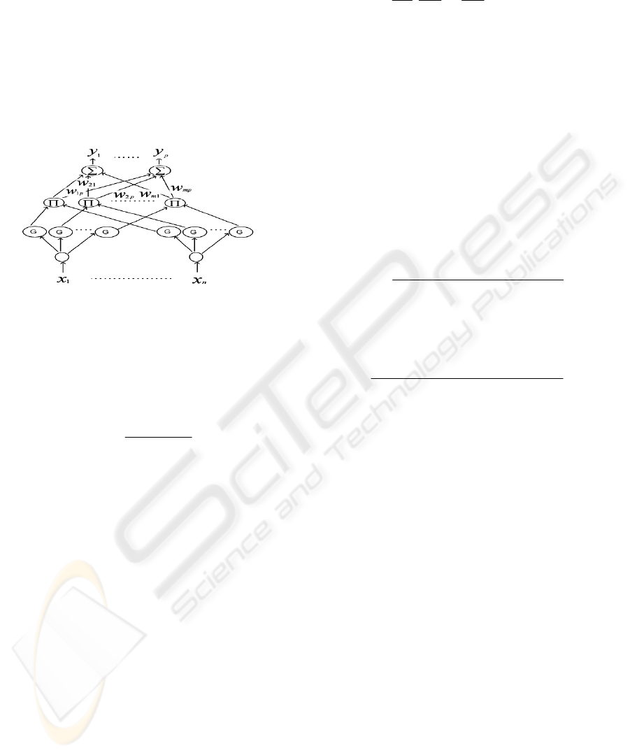
diagram of the proposed RFNN structure is shown in

Fig. 1 which indicates the signal propagation and the

operation functions of the nodes in each layer. In the

following description,

u denotes i-th input of a

node in the k-th layer;

denotes the i-th node

output in the k-th layer. For the sake of brevity, a

brief description of the RFNN is introduced.

Interested readers are referred to reference (Lee,

2005).

Figure 1: structure of RFNN.

Layer 1: Input Layer:

uo =

(1)

Layer 2: Membership Layer: The Gaussian function

is adopted here as a membership function:

⎪

⎭

⎪

⎬

⎫

⎪

⎩

⎪

⎨

⎧

−

−=

)(

exp

(2)

where

m and

are the center (or mean) and the

width (or standard deviation—STD) of the Gaussian

membership function. The subscript ij indicates the

j-th term of the i-th input. In addition, the inputs of

this layer for discrete time k can be denoted by

)()()(

kokoku

iij

(3)

where

ijij

koko

×−= )1()(

and

denotes the link

weight of the feedback unit. It is clear that the input

of this layer contains the memory terms

)1(

−

which store the past information of the network.

Each node in this layer has three adjustable

parameters:

m ,

, and

Layer 3: Rule Layer:

[][]

⎭

⎬

⎫

⎩

⎨

⎧

−−−

∏

)()(exp

muDmuD

(4)

Where

[][ ]

niiii

niii

mmmmuuuu

diagD

,...,,,,...,,

,...,

2121

⎭

⎬

⎫

⎩

⎨

⎧

σσσ

(5)

Layer 4: Output Layer:

∑

jpjpp

wuoy

444

(6)

where

and

(the link weight) is the output

action strength of the i-th output associated with the

j-th rule.

w are the tuning factors of this layer.

Finally, the overall representation of input x and the

p-th output is

⎥

⎦

⎤

⎢

⎣

⎡

−×−+

−

×==

∏

∑

)(

))1()((

exp

)(

ijij

mkokx

woky

(7)

Where

⎥

⎦

⎤

⎢

⎣

⎡

−×−+−

−

=−

)(

))2()1((

exp

)1(

ijij

mkokx

(8)

Obviously, using the RFNN, the same inputs at

different times yield different outputs. The proposed

RFNN can be shown to be a universal uniform

approximator for continuous functions over compact

sets if it satisfies a certain condition (Lee, 2000).

3 BPSO

With correct combination of GA and PSO, the

hybrid can outperform, or perform as well as, both

the standard PSO and GA models (

Settles, 2005). The

hybrid algorithm combines the standard velocity and

position update rules of PSOs with the ideas of

selection, crossover and mutation from GAs. An

additional parameter, the breeding ratio (Ψ),

determines the proportion of the population which

undergoes breeding (selection, crossover and

mutation) in the current generation. Values for the

breeding ratio parameter range from (0.0:1.0).

In each generation, after the fitness values of all

the individuals in the same population are

calculated, the bottom (N · Ψ) are discarded and

removed from the population where N is the

population size. The remaining individual’s velocity

vectors are updated, acquiring new information from

COMBINATION OF BREEDING SWARM OPTIMIZATION AND BACKPROPAGATION ALGORITHM FOR

TRAINING RECURRENT FUZZY NEURAL NETWORK

315

the population. The next generation is then created

by updating the position vectors of these individuals

to fill (N · (1 − Ψ)) individuals in the next

generation. The (N · Ψ) individuals needed to fill the

population are selected from the individuals whose

velocity is updated to undergo VPAC crossover and

mutation and the process is repeated. For clarity, the

flow of these operations is illustrated in Figure 1

where k = (N · (1 − Ψ)).

Figure 2: BPSO.

Here, we developed crossover operator to utilize

information available in the Breeding Swarm

algorithm, but not available in the standard GA

implementation. The new crossover operator,

velocity propelled averaged crossover (VPAC),

incorporates the PSO velocity vector. The goal is

creating two new child particles whose position is

between the parent’s positions, but accelerated away

from the parent’s current direction (negative

velocity) in order to increase diversity in the

population. Equations (8) show how the new child

position vectors are calculated using VPAC.

⎪

⎩

⎪

⎨

⎧

−

)(

0.2

)()(

)(

0.2

)()(

)(

xpxp

(9)

In these equations,

)(

1 i

and

)(

2 i

are the

positions of child 1 and 2 in dimension i,

respectively.

)(

1 i

and

)(

2 i

are the positions of

parents 1 and 2 in dimension i, respectively.

)(

1 i

and

)(

2 i

are the velocities of parents 1 and 2 in

dimension i, respectively.

is a uniform random

variable in the range [0.0:1.0]. Towards the end of a

typical PSO run, the population tends to be highly

concentrated in a small portion of the search space,

effectively reducing the search space. With the

addition of the VPAC crossover operator, a portion

of the population is always pushed away from the

group, increasing the diversity of the population and

the effective search space.

The child particles retain their parents’s velocity

vector

),()(

vpvc

)()(

vpvc

. The previous

best vector is set to the new position vector,

restarting the child’s memory by replacing new

)()(),()(

2211

xppcxppc

. The velocity and

position update rules remain unchanged from the

standard inertial implementation of the PSO. The

social parameters are set to 2.0 while inertia is

linearly decreased from 0.7 to 0.4 and a maximum

velocity (Vmax) of ±1 was allowed. The breeding

ratio was set to an arbitrary 0.3. Tournament

selection, with a tournament size of 2, is used to

select individuals as parents for crossover. The used

mutation operator is Gaussian mutation, with mean

0.0 and variance reduced linearly in each generation

from 1.0 to 0.0. Each weight in the chromosome has

probability of mutation 0.1.

4 NETWORK TRAINING

BP approach, as mentioned, has been mostly used

for training RFNN in previous works. This approach

is not easy to implement, when faced with the case

of a complete or a non-diagonal fuzzy rule base. As

we can see in Fig. 1, each rule of layer 3 is made by

only a diagonal variables, i.e. the i-th rule are made

by multiplication of the i-th outputs of layer 2.

However, if we want to use complete or non-

diagonal fuzzy rule base, it will make learning of

parameters in layer 2 totally complicated. In this

paper we propose Breeding Particle Swarm

Optimization for tuning parameters of layer 2

(

) and original BP for tuning

. These

two approaches are used simultaneously. Pseudo

code of the algorithm used in this study for training

RFNN parameters is shown in Fig. 3. The proposed

combination has various benefits for training RFNN.

First of all, there is no need to differentiate those

complex derivations for training the parameters of

the 2

layer. The proposed algorithm utilizes BPSO

as a derivative-free approach for training these

parameters. The method is also a global optimization

approach that prevents training parameters from

converging to local minima. Because of simplicity

and high speed convergence, the parameters of 4

layer is learned by BP. Note that using a complete

fuzzy rule base doesn’t affect the tuning of

BP and will not increase its complexity.

ICINCO 2008 - International Conference on Informatics in Control, Automation and Robotics

316

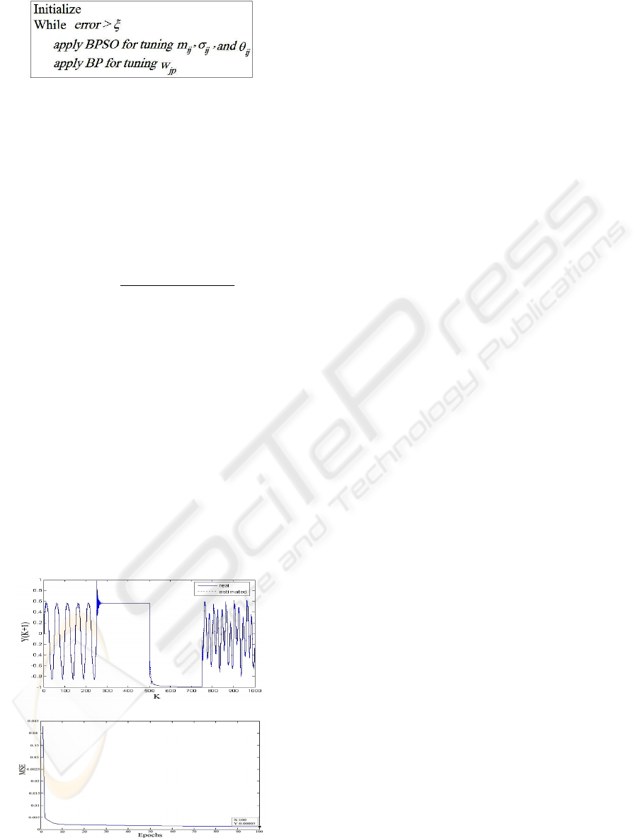
Figure 3: Pseudo code of the proposed tuning algorithm.

5 SIMULATION RESULTS

Suppose the following nonlinear dynamical system:

))1(),(),2(),1(),((

)1(

−−−

kukukykykyf

ppp

(10)

Where,

435321

54321

)1(

),,,,(

xxxxxx

xxxxxf

+−

(11)

In this system the output value depended on the

previous values of the output and the previous

values of the input. We use RFNN to identify this

system. Because of dynamical characteristics of

RFNN, it is not necessary to use all complete

samples of the previous inputs and outputs. So just

y(k) and u(k) are used for estimating y(k+1). The

parameters of the 2nd layer of the RFNN is tuned by

BPSO and the output weights,

is tuned with BP

simultaneous. The same input signal that was used in

(Lee, 2000) is used here for testing. Fig. 4 illustrates

that learning of the network is successfully done.

This method leads to better identification than the

previous ones. The MSE parameter was 0.00013 in

original method while our proposed method

converges to 0.00005.

Figure 4: training RFNN parameters with cooperation of

the BPSO and BP. a) Identification. b) MSE.

6 CONCLUSIONS

In this study a novel approach for training RFNN

was proposed. BP algorithm suffers from complexity

of differentiating and converging to local minima.

Our proposed method utilizes BPSO with

combination of BP. As the simulation results show,

applying this algorithm improves the performance of

training RFNN. This improvement is gained by

globally optimizing the feature of PSO that prevents

training to be entrapped in local minima. The

complexity of differentiating for gradient based

methods is more serious when a complete or a non-

diagonal fuzzy rule base is used. This algorithm

solves this problem too and one can use it more

frequently.

REFERENCES

Angeline, P., Saunders, G., Pollack, J.,1994. An

evolutionary algorithm that constructs recurrent neural

networks.

Engelbrecht, A. P., 2002. Computational Intelligence.

John Wiley and Sons,2002.

Kennedy, J., Eberhart, R., 1995. Particle Swarm

Optimization. IEEE International Conference on

Neural Networks , pp. 1942-1948.

Ku, C. C., Lee, K. Y., 1995. Diagonal recurrent neural

networks for dynamic systems control. IEEE Trans.

Neural Networks, vol. 6, pp. 144–156.

Lee, C. H., Teng, C., 2000. Identification and Control of

Dynamic Systems Using Recurrent Fuzzy Neural

Networks. In IEEE Transactions on fuzzy systems,

vol.8, NO. 4, 349,366 .

Settles, M., Nathan, P., Soule, T, 2005. Breeding Swarms:

A New Approach to Recurrent Neural Network

Training. GECCO’05, June 25–29 Washington, DC,

USA.

Soule, T., Chen, Y., Wells, R.,2002. . Evolving a strongly

recurrent neural network to simulate biological eurons.

In the proceedings of The 28th Annual Conference of

the IEEE Industrial Electronics Society.

Surmann, H., Maniadakis, M., 2001. Learning feed-

forward and recurrent fuzzy systems: A genetic

approach. Journal of System Architecture 47, 649-662.

Williams, R. J., Zipser, D.,1989. A learning algorithm for

continually running fully recurrent neural networks.

Neural Computation., vol. 1, pp. 270–280.

COMBINATION OF BREEDING SWARM OPTIMIZATION AND BACKPROPAGATION ALGORITHM FOR

TRAINING RECURRENT FUZZY NEURAL NETWORK

317