A GUARANTEED STATE BOUNDING ESTIMATION FOR
UNCERTAIN NON LINEAR CONTINUOUS TIME SYSTEMS USING
HYBRID AUTOMATA
Nacim Meslem, Nacim Ramdani and Yves Candau
CERTES EA 3481 Universit
´
e Paris 12-Val de Marne, 61 av. G. de Gaulle, Cr
´
eteil, France
INRIA Sophia Antipolis - M
´
editerran
´
ee - Antenne de Montpellier (LIRMM)
161 rue Ada - 34392 Montpellier cedex, France
Keywords:
State estimation, non linear systems, bounded error context, non linear differential equations, interval analysis,
guaranteed numerical integration, hybrid automata.
Abstract:
This work is about state estimation in the bounded error context for non linear continuous time systems. The
main idea is to seek to estimate not an optimal value for the unknown state vector but the set of feasible values,
thus to characterize simultaneously the value of the vector and its uncertainty. Our contribution resides in the
use of comparison theorems for differential inequalities and the analysis of the monotonicity of the dynamical
systems with respect to the uncertain variables. The uncertain dynamical system is then bracketted between
two hybrid dynamical systems. We show how to obtain this systems and to use them for state estimation with
a prediction-correction type observer. An example is given with bioreactors.
1 INTRODUCTION
State estimation with continuous dynamic systems is
recognized as problem of great importance in prac-
tice. Indeed, to apply advanced methods for the con-
trol or the diagnosis of dynamical systems one often
needs to compute on-line their internal state. Gener-
ally the direct measurement of this state by means of
sensors may not be available for various reasons such
as physical, practical, economic, . . . etc. However, it
is possible to carry out this task by software sensors,
i.e. observers or estimator which can provide on line
an estimate of the real state system, under certain con-
ditions of observability (Hermann and J.Krener, 1977;
Hermann, 1963).
In fact, there are always uncertainties in the math-
ematical models used for characterizing the system
under study. Consequently, the classical approaches
for building observers are insufficient (Dochain,
2003). Thus, a new approach was developed recently
in a deterministic set-membership context, which
aims to reconstruct all the state trajectories which are
consistent with both the uncertain models and the un-
certain measurements.
This approach can be used easily when mea-
surements are available at discrete time. It is of
prediction-correction type: (i) The prediction phase
consists in computing a guaranteed over (conserva-
tive) approximation of the reachable state space gen-
erated by the uncertain system, (ii) and the correction
phase consists in removing from this over approxima-
tion all the part which are not consistent with feasible
measurements domains, each time a measurement is
available.
In the literature, several geometrical forms are
used to implement this set-membership approach with
linear systems. For example, parallelotopes (Chisci
et al., 1996), ellipsoidal (Chernousko, 2005) and
zonotopes (Combastel, 2005).
With nonlinear systems, guaranteed numerical in-
tegration method for the ordinary differential equation
(ODE) (Nedialkov, 1999) based on intervals Taylor
models (Moore, 1966) was used recently to solve this
estimation problem (Ra
¨
ıssi et al., 2004). Generally,
the wrapping effect (Moore, 1966; Nedialkov, 1999)
associated with the intervals representation of uncer-
tain variables limits considerably their use in order to
deal with practical cases. Thereafter, in order to cir-
cumvent the wrapping effect, the authors of (Kieffer
and Walter, 2006) used the M
¨
uller’s existence theo-
rem (M
¨
uller, 1926; Walter, 1997) as a tool for deriv-
ing a guaranteed enclosure for an uncertain dynami-
32
Meslem N., Ramdani N. and Candau Y. (2008).
A GUARANTEED STATE BOUNDING ESTIMATION FOR UNCERTAIN NON LINEAR CONTINUOUS TIME SYSTEMS USING HYBRID AUTOMATA.
In Proceedings of the Fifth International Conference on Informatics in Control, Automation and Robotics - SPSMC, pages 32-37
DOI: 10.5220/0001490400320037
Copyright
c
 SciTePress

cal system between two deterministic dynamical sys-
tems. The main difficulty resides in the definition of
the bracketing systems. Our contribution is in the con-
tinuation of these work since we show how to build
deterministic hybrid dynamical systems as bracketing
systems and thus make it possible to use the M
¨
uller
theorem with a larger class of nonlinear dynamical
systems.
This work is organized as flow. In the second
section we present the context and the main ideas of
set-membership estimation. Then, we will recall the
M
¨
uller’s theorem in section 3. We introduce the hy-
brid bracketing approach for uncertain dynamical sys-
tems in section 4. Finally we illustrate our method on
a model drawn from bioreactors domain in section 5.
2 PROBLEM STATEMENT
2.1 Context
Let us consider the uncertain continuous dynamic sys-
tem (1) where uncertainties are naturally represented
by bounded intervals with a priori known bounds,





˙
x(t) = f(x,u,[p],t)
y(t) = g(x,u,[p],t)
x(t
0
) ∈ [x
0
] ⊂ D





(1)
where t ∈[t
0
,T ], f ∈C
k−1
(D ×U ×[p]), D ×U ×[p] ⊆
R
n+n
u
+n
p
is an open set; n, n
u
, m and n
p
are the di-
mension of respectively the state vector x, the input
vector u, the output vector y and the parameter vec-
tor p. The functions f : D ×U ×[p] → R
n
and h :
D ×U ×[p] → R
m
are possibly nonlinear. The initial
state x
0
is assumed to belong to a prior known set [x].
We assume that measurements y
j
of the output vec-
tor are available at sampling times t
i
∈ {t
1
,t
2
,...,t
n
}
in I = [t
0
,t
n
T
]. Note that the sampling interval needs
not be constant. The measurement noise is a dis-
crete time signal assumed additive and bounded with
known bounds. Denote E
j
a feasible domain for out-
put error at time t
j
: the feasible domain for model
output at time t
j
is then given by
Y
j
= y
j
+ E
j
(2)
Under these considerations, estimating the state
vector x consists in determining an upper approxima-
tion of the set X(t) of all acceptable state trajectories
X(t) =





x(t) | (∀t ∈ I
˙
x(t) = f(x,u,[p],t))
∧
(∀t
j
∈ {t
1
,t
2
,...,t
nT
},
x(t
j
) ∈ (g
−1
(Y(t
j
),u,[p]) ∩[x
j
]))





(3)
j




x
1j
+
+


x
()
f
=xx

()
1
1j
gy
−
+


Figure 1: Prediction and correction phases.
2.2 Principle: Prediction-correction
Method
Figure 1 shows the principle of the prediction and
correction phases for this set-membership approach,
between two successive time measurement indexes t
j
and t
j+1
. Indeed, by using one of the guaranteed nu-
merical simulation methods for uncertain ODEs, the
prediction phase computes an guaranteed over enclo-
sure [x
j+1
]
p
for all solutions of (1) at the time t
j+1
with (t
j
, [x
j
]) as initial conditions.
x(t
j+1
;t
j
,[x
j
]) ⊆ [x
j+1
]
p
. (4)
The correction phase uses set inversion, consis-
tency techniques and intervals analysis (Jaulin et al.,
2001) to characterize the reciprocal image [x
j+1
]
inv
at time t
j+1
of the admissible measurement domain
Y
j+1
by the output model g
[x
j+1
]
inv
= g
−1
([y
j+1
],[p]) (5)
where [y
j+1
] = Y
j+1
.
Thereafter, it contracts the predicted state inter-
vals vector by comparing it with the reciprocal image
[x
j+1
]
inv
and eliminating the inconsistent state vectors
[x
j+1
]
c
= [x
j+1
]
inv
∩[x
j+1
]
p
(6)
Thus for the next measurement the predication
phase will be initialized by [x
j+1
] = [x
j+1
]
c
. In fact,
by repeating these two phases each time a new mea-
surement is available, one improves considerably pre-
cision of the guaranteed over approximation of the set
X(t).
The algorithm below shows the process for this
set-membership estimation approach
A GUARANTEED STATE BOUNDING ESTIMATION FOR UNCERTAIN NON LINEAR CONTINUOUS TIME
SYSTEMS USING HYBRID AUTOMATA
33

Algorithm : Prediction Correction estimation
1. Input: ([x
0
],[p], f,g, [y
1
],. .. ,[y
nT
])
2. t
j
= t
0
; [x
j
] = [x
0
];
3. while (t
j
< t
nT
) do
4. {t
j+1
,[x
j+1
]
p
}=Validated Integration([x
j
],[p],t
j
);
5. [x
j+1
]
inv
= g
−1
([y
j+1
],[p]);
6. [x
j+1
]
c
= [x
j+1
]
inv
∩[x
j+1
]
p
;
7. [x
j+1
] = [x
j+1
]
c
8. j = j + 1;
9. end
10. Output: X(t).
3 M
¨
ULLER’S THEOREM
In this section, we introduce an approach for brack-
eting an uncertain dynamical systems when both the
initial state and parameter vectors are defined by
boxes (intervals vector). The main idea consists in
building a lower and an upper dynamical system
which involve no uncertainty and enclose in a guar-
anteed way, the all state trajectories generated by
the original uncertain system. This approach relies
on comparison theorems for differential inequalities
(Smith, 1995; Hirsch and Smith, 2005), and in partic-
ular the work of M
¨
uller (M
¨
uller, 1926; Marcelli and
Rubbioni, 1997).
Theorem:(M
¨
uller, 1926; Kieffer and Walter, 2006)
Consider the dynamical system
˙
x(t) = f(x,p,u(t)), (7)
where function f is continuous over a domain T de-
fined by
T :





ω(t) ≤ x(t) ≤ Ω(t)
p ≤ p ≤ p
t
0
≤t ≤t
n
T
(8)
Functions ω
i
(t) and Ω
i
(t) are continuous over [t
0
,t
n
T
]
for all i and satisfy the following properties
1. ω(t
0
) = x
0
and Ω(t
0
) = x
0
2. the left derivatives D
−
ω
i
(t) and D
−
Ω
i
(t) and the
right derivatives D
+
ω
i
(t) and D
+
Ω
i
(t) of ω
i
(t)
and Ω
i
(t) are such that
∀i, D
±
ω
i
(t) ≤ min
T(t)
f
i
(x,p,t) (9)
∀i, D
±
Ω
i
(t) ≥ max
T(t)
f
i
(x,p,t) (10)
where T(t) is the subset of T(t) defined by
T
i
:





x
i
= ω
i
(t)
ω
j
(t) ≤ x
j
≤ Ω
j
(t), j 6= i
p ≤ p ≤ p
(11)
and where T(t) is the subset of T(t) defined by
T
i
:





x
i
= Ω
i
(t)
ω
j
(t) ≤ x
j
≤ Ω
j
(t), j 6= i
p ≤ p ≤ p
(12)
Then for all x
0
∈[x
0
,x
0
], p ∈[p,p], system (1) admits
a solution x(t) that stays in the domain
X :

t
0
≤t ≤t
n
T
ω(t) ≤ x(t) ≤ Ω(t)
(13)
and takes the value x
0
at t
0
. If, in addition, for all p ∈
[p
0
,p
0
], function f(x, p,t) is Lipschitzian with respect
to x over D then this solution is unique for any given
p.
Finally, an enclosure for the solution of (7) is
given by
∀t ∈ [t
0
, t
n
T
], [x](t) = [ω(t), Ω(t)] (14)
The main difficulty is to obtain suitable bracketing
functions ω(t) and Ω(t) in the general case. However,
when the components of f are monotonic with respect
to each parameter and each state vector component,
it is quite easy to define these systems (Kieffer et al.,
2006), while avoiding possible divergence that may
occur when both upper and lower components of the
parameter/state vector appear simultaneously in the
same expression of the components of the bracketing
systems (Ramdani et al., 2006).
Rule 1 - Use of monotonicity property (Kieffer et al.,
2006)
In order to build the upper system, i.e. the one which
yields the upper solution Ω(t), one can replace in the
formal expression of f
i
, x
i
by Ω
i
, x
j
( j 6= i) by Ω
j
if
∂ f
i
∂x
j
≥ 0 or by ω
j
if
∂ f
i
∂x
j
≤ 0 and p
k
by p
k
if
∂ f
i
∂p
r
≥ 0 or
by p
k
if
∂ f
i
∂p
k
≤ 0. The components of the lower sys-
tem, i.e. the one which yields the lower solution ω(t)
are derived by reversing monotonicity conditions.
Obviously ω(t) and Ω(t) are in general, solutions
of a system of coupled differential equations, i.e.











˙
ω(t) = f(ω,Ω,p,p,t)
˙
Ω(t) = f(ω,Ω,p,p,t)
ω(t
0
) = x
0
Ω(t
0
) = x
0
(15)
which involves no uncertain quantity. Therefore in-
terval Taylor models such as the one presented in (Ne-
dialkov, 1999) can be used for efficiently solving (15).
Indeed when these methods are used for solving dif-
ferential equations with no uncertainty, they are usu-
ally able to curb the pessimism induced by the wrap-
ping effect, even over long integration time.
ICINCO 2008 - International Conference on Informatics in Control, Automation and Robotics
34

4 HYBRID BRACKETING
SYSTEM
Now, one address the case of uncertain dynamical
systems (1), for which the signs of the partial deriva-
tives ∂ f
i
/∂p
k
and ∂ f
i
/∂x
j
change along the integra-
tion time interval [t
0
,t
n
T
]. In such a case, the uncertain
system (1) admits an enclosure over each time inter-
val where functions f
i
are monotonic with respect to
variables p
k
and x
j
. Therefore both upper and lower
bounding systems are defined by piecewise nonlinear
ODEs and can thus be regarded as hybrid dynamical
systems. Thus, they can be modeled by an hybrid au-
tomaton(Alur et al., 1995).
So to compute a guaranteed enclosure of reach-
able state space generated by the uncertain system (1),
we will built hybrid system of l continuous dynamic
modes which satisfied locally conditions imposed by
rule 1
M = {M
1
,M
2
,...,M
l
} (16)
and which given in state space representation by
(
˙
ω(t) = f
M
i
(ω,Ω,p,p,t)
˙
Ω(t) = f
M
i
(ω,Ω,p,p,t)
for i = 1,...,l (17)
Hence, the evolution of this hybrid system is con-
trolled by the sign changes of the partial derivatives
∂ f
i
/∂p
k
and ∂ f
i
/∂x
j
which represents the guard con-
ditions which authorize the transitions between the
continuous bracketing modes. Thus, for a given ini-
tial conditions the execution of this hybrid automata
makes it possible to obtain a guaranteed upper ap-
proximation of the reachable state space of the con-
tinuous time system (1).
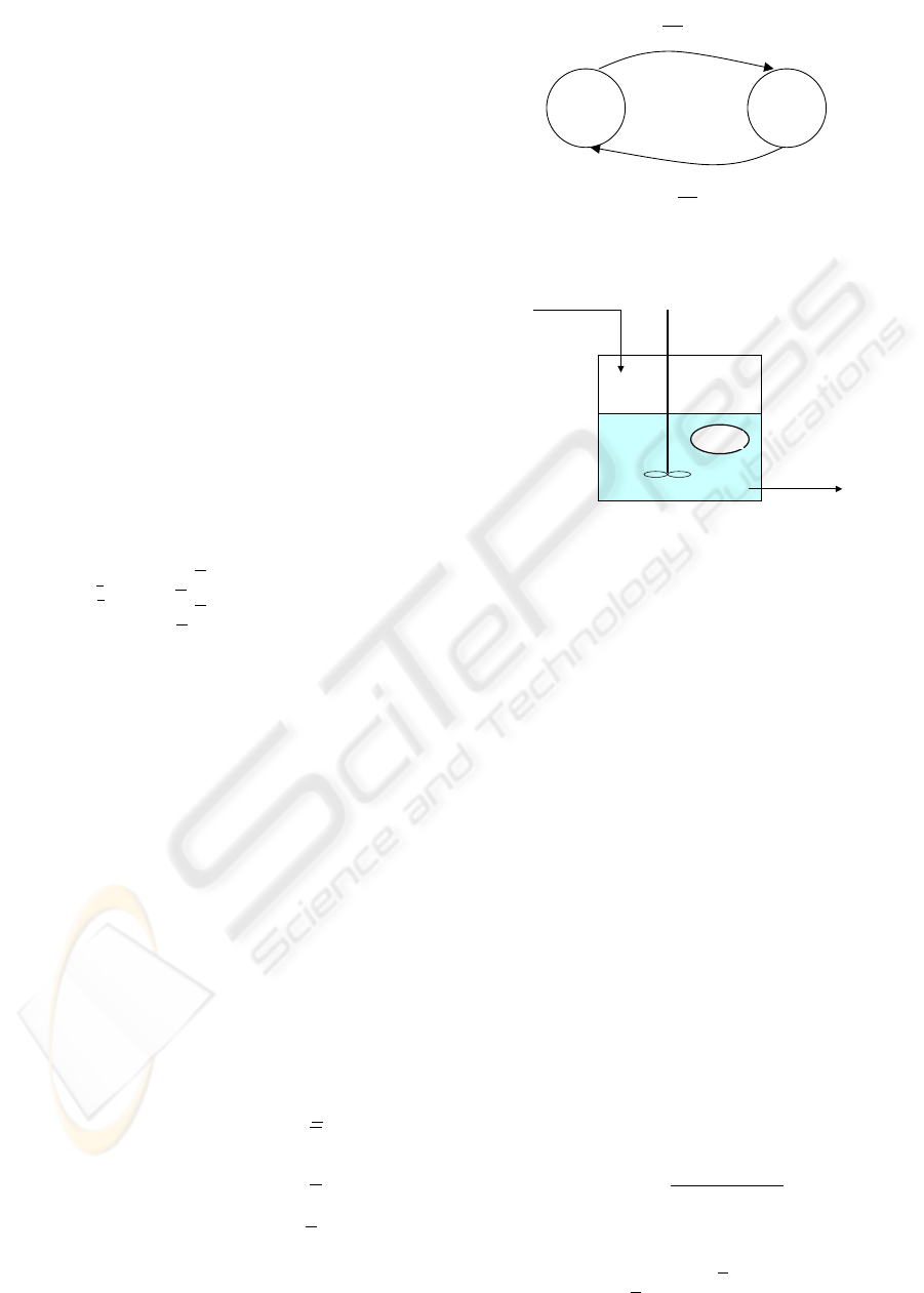
Example:
Let us consider the following system
˙x(t) = f (x,[p]). (18)
According to the sign of ∂ f /∂p, the system (18)
admitted two possible bracketing modes
i f ∂ f /∂p ≤0
then M
1
=

˙
Ω(t) = f
M
1
(Ω, p
)
˙
ω(t) = f
M
1
(ω, p)
(19)
else M
2
=

˙
Ω(t) = f
M
2
(Ω, p)
˙
ω(t) = f
M
2
(ω, p).
(20)
and its hybrid bracketing automata is represented in
the figure 2
0
∂
>
∂
f
p
M
1
M
2
0
∂
≤
∂
f
p
Figure 2: Hybrid automata.
Fou
t
Fin, Sin
X
,
S
Figure 3: General representation of a bioreactor.
5 APPLICATION
5.1 Model
Generally, the mathematical model of biotechnolog-
ical processes is difficult to establish with accuracy,
that is due to the living behavior of the bacteria rep-
resented by a complex poorly known function of the
bioreactor state. In this section we consider a simple
model where only one population of bacteria is taken
into account. In this context, to describe the state of
the bioreactor, two state variables are necessary, the
first one represents the bacteria concentration called
biomass and denoted X, the second one represents the
substrate concentration, denoted S. Thus the model
below shows the evolution of the biomass by consum-
ing the polluting body S

X(t) = µ(S)X −αDX
S(t) = −k
1
µ(S)X + D(S
in
−S)
(21)
where µ(s) is the growth rate of biomass modeled by
the Haldane law:
µ(S) = µ
0
S
S + k
s
+ S
2
/k
i
(22)
with the uncertain bounded parameter µ
0
µ
0
≤ µ
0
≤ µ
0
.
A GUARANTEED STATE BOUNDING ESTIMATION FOR UNCERTAIN NON LINEAR CONTINUOUS TIME
SYSTEMS USING HYBRID AUTOMATA
35

This bioreactor is fed by a solution containing sub-
strate in concentration S
in
which is not exactly mea-
sured
S
in
(t) ≤ S
in
(t) ≤ S
in
(t)
and we suppose that the biomass is accessible to mea-
surement
y(t) = X(t).
5.2 Building Hybrid Bracketing System
For this application, according to the sign of the
derivative of µ with respect to S,
sign(
dµ(S)
dS
)



> 0 if S <
√
k
s
k
i
, ∀S ∈[S]
≤ 0 if S ≥
√
k
s
k
i
, ∀S ∈[S]
ambiguous if
√
k
s
k
i
∈ [S]
(23)
system (21) allows three possible modes for the
bracketing. The first mode, M
1
= 1, corresponds to
the intervals time when this derivative is negative
(M
1
= 1)







X(t) = µ(S)X −αDX
S(t) = −k
1
µ(S)X + D(S
in
−S)
X(t) = µ(S)X −αDX
S(t) = −k
1
µ(S)X + D(S
in
−S)
(24)
and the second mode, M
2
= 2, is linked to intervals
time where this derivative is positive
(M
2
= 2)







X(t) = µ(S)X −αDX
S(t) = −k
1
µ(S)X + D(S
in
−S)
X(t) = µ(S)X −αDX
S(t) = −k
1
µ(S)X + D(S
in
−S).
(25)
Finally, the third mode M
3
= 0 is associated to case
when the sign of this derivative is ambiguous. In this
case either one uses guaranteed integration methods
based on interval Taylor models to bracket (21), or if
this is possible, one finds a trivial bracketing for µ(s).
For example,
µ
0
S
S + k
s
+ SS/k
i
≤ µ(S) ≤ µ
0
S
S + k
s
+ SS/k
i
.
Hence, one propose the below differential equations
system for the third mode M
3
= 0
(M
3
= 0)









X(t) = µ
0
S
S+k
s
+SS/k
i
X −αDX
S(t) = −k
1
µ(S)X + D(S
in
−S)
X(t) = µ
0
S
S+k
s
+SS/k
i
X −αDX
S(t) = −k
1
µ(S)X + D(S
in
−S).
(26)
Now, function Validated Integration in algo-
rithm Prediction Correction Estimation selects on
line the local bracketing mode according to the sign
of
dµ(.)
dS
and then uses guaranteed numerical integra-
tion methods for ODE based on intervals Taylor mod-
els for solving (24), (25) or (26).
5.3 Results of Simulation
The data considered in this example are as fol-
lows: α = 0.5, k = 42.14, k
s
= 9.28mmol/l, k
i
=
256mmol/l, µ
0
∈ [0.64,0.84], X
0
∈ [0 >,10], S
0
∈
[0,100], S
in
(t) ∈ ([62,68] + 15 cos(1/5t)),
D(t) =



2 si 0 ≤t ≤ 5
0.5 si 5 ≤t ≤ 10
1.14 si 10 ≤t ≤ 20,
and the feasible measurement domain
Y(t
j
) = [0.98y
m
(t
j
),1.02y
m
(t
j
)]
with a constant measurements time step t
j+1
−t
j
= 2.
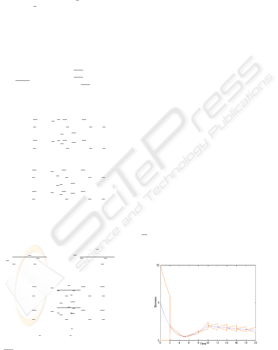
The red continuous lines curves in figures 4 and
5 show the guaranteed enclosure of all the possible
state trajectories of (21) which are compatible with
the model and its uncertainties and the acceptable do-
main of the discrete measurements signal. The dis-
continuous blue curves represent the real state of (21)
which corresponds to the following values of the un-
certain parameters and the initial state: µ
0
= 0.74,
X
0
= 5, S
0
= 40 and S
in
(t) = 65 + 15 cos(1/5t).
So figure 6 shows the actual commutations be-
tween the three bracketing modes as obtained during
the simulation period. This represents the evolution of
the discrete component of the hybrid automata used to
bracket the state flow generated by the uncertain sys-
tem (21).
As a conclusion, guaranteed numerical integration
methods for ODE based on the interval Taylor mod-
els fail to give non divergent enclosures after few inte-
gration step because of the large magnitude in uncer-
tainty in both parameter vector and initial state vector.
In addition, rule 1 is not applicable over all the simu-
lation period because the sign of the partial derivative
∂
˙
X
∂S
changes with time. Hence, our hybrid bracketing
method is an important alternative to solve set mem-
bership estimation problems of this kinds.
Figure 4: The both real and estimated evolution the
biomass.
ICINCO 2008 - International Conference on Informatics in Control, Automation and Robotics
36

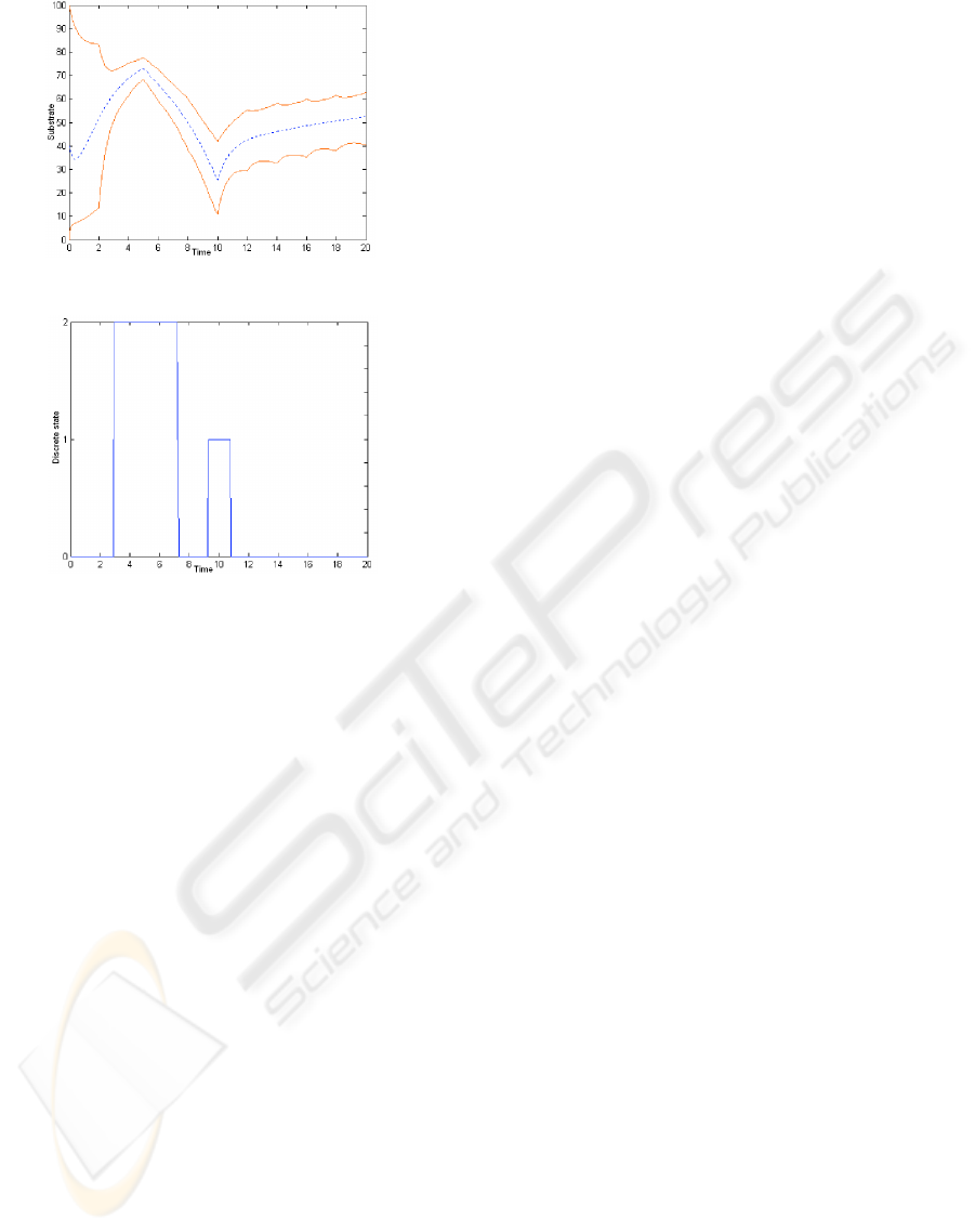
Figure 5: The both real and estimated evolution the sub-
strate.
Figure 6: Indices of the three bracketing modes used over
the simulation period.
6 CONCLUSIONS
In this communication, we wanted to show that by us-
ing the M
¨
uller’s theorem and by analyzing the mono-
tonicity of the uncertain dynamical system with re-
spect to both the uncertain variables and parameters,
one is able to solve the state membership estimation
problem for a large class of uncertain dynamical sys-
tems. Indeed, the method presented makes it possi-
ble to circumvent the propagation of the pessimism
due to the wrapping effect which generally causes the
divergence of guaranteed numerical integration meth-
ods based on interval Taylor models when used with
uncertain ODEs. In the future, we wish to extend this
approach for systems with higher dimension and also
to hybrid dynamical systems.
REFERENCES
Alur, R., Courcoubetis, C., Halbwachs, N., Henzinger, T.,
Ho, P.-H., Nicollin, X., Olivero, A., Sifakis, J., and
Yovine, S. (1995). The algorithmic analysis of hybrid
systems. Theoretical Computer Science, 138:3–34.
Chernousko, F. (2005). Ellipsoidal state estimation for dy-
namical systems. Nonlinear analysis.
Chisci, L., Garulli, A., and Zappa, G. (1996). Recur-
sive state bounding by parallelotopes. Automatica,
32:1049–1055.
Combastel, C. (2005). A state bounding observer for un-
certain nonlinear continuous-time systems based on
zonotopes. In 44th IEEE Conference on decision and
control and European control conference ECC 2005.
Dochain, D. (2003). State and parameter estimation in
chemical and biochemical processes: a tutorial. Jour-
nal of process control, 13:801–818.
Hermann, R. (1963). On the accessibility problem in control
theory. In in Int. Symp. on nonlinear differential equa-
tions and nonliear mechanics, pages 325–332, New
York. Academic Press.
Hermann, R. and J.Krener, A. (1977). Nonlinear control-
lability and observability. Transactions on Automatic
Control, AC-22:728–740.
Hirsch, M. and Smith, H. (2005). Monotone dynamical sys-
tems. In Canada, A., Drabek, P., and Fonda, A., ed-
itors, Handbook of Differential Equations, Ordinary
Differential Equations, volume 2, chapter 4. Elsevier.
Jaulin, L., Kieffer, M., Didrit, O., and Walter, E. (2001).
Applied interval analysis: with examples in parame-
ter and state estimation, robust control and robotics.
Springer-Verlag, London.
Kieffer, M. and Walter, E. (2006). Guaranteed nonlinear
state estimation for continuous-time dynamical mod-
els from discrete-time measurements. In Proceedings
6th IFAC Symposium on Robust Control, Toulouse.
Kieffer, M., Walter, E., and Simeonov, I. (2006). Guaran-
teed nonlinear parameter estimation for continuous-
time dynamical models. In Proceedings 14th IFAC
Symposium on System Identification, pages 843–848,
Newcastle, Aus.
Marcelli, C. and Rubbioni, P. (1997). A new extension of
classical m
¨
uller theorem. Nonlinear Analysis, Theory,
Methods & Applications, 28(11):1759–1767.
Moore, R. (1966). Interval analysis. Prentice-Hall, Engle-
wood Cliffs.
M
¨
uller, M. (1926). Uber das fundamentaltheorem in
der theorie der gew
¨
ohnlichen differentialgleichungen.
Math. Z., 26:619–645.
Nedialkov, N. (1999). Computing rigorous bounds on the
solution of an initial value problem for an ordinary
differential equation. PhD University of Toronto.
Ra
¨
ıssi, T., Ramdani, N., and Candau, Y. (2004). Set mem-
bership state and parameter estimation for systems de-
scribed by nonlinear differential equations. Automat-
ica, 40(10):1771–1777.
Ramdani, N., Meslem, N., Ra
¨
ıssi, T., and Candau, Y.
(2006). Set-membership identification of continuous-
time systems. In Proceedings 14th IFAC Symposium
on System Identification, pages 446–451, Newcastle,
Aus.
Smith, H. (1995). Monotone dynamical systems: An intro-
duction to the theory of competitive and cooperative
systems. Ams. providence, ri edition.
Walter, W. (1997). Differential inequalities and maximum
principles: Theory, new methods and applications.
Nonlinear Analysis, Theory, Methods & Applications,
30(8):4695–4711.
A GUARANTEED STATE BOUNDING ESTIMATION FOR UNCERTAIN NON LINEAR CONTINUOUS TIME
SYSTEMS USING HYBRID AUTOMATA
37