FAULT DETECTION BY MEANS OF DCS ALGORITHM
COMBINED WITH FILTERS BANK
Application to the Tennessee Eastman Challenge Process
Oussama Mustapha, Mohamad Khalil
Lebanese University, Faculty of Engineering, Section I- El Arz Street, El Kobbe, Lebanon
Islamic University of Lebanon, Biomedical Department, Khaldé, Lebanon
Ghaleb Hoblos, Houcine Chafouk
ESIGELEC, IRSEEM, Saint Etienne de Rouvray, France
Dimitri Lefebvre
GREAH – University Le Havre, France
Keywords: Signal processing, Filters Bank, Dynamic Cumulative Sum, Fault detection, Chemical processes.
Abstract: Early fault detection, which reduces the possibility of catastrophic damage, is possible by detecting the
change of characteristic features of the signals. The aim of this article is to detect faults in complex
industrial systems, like the Tennessee Eastman Challenge Process, through on-line monitoring. The faults
that are concerned correspond to a change in frequency components of the signal. The proposed approach
combines the filters bank technique, for extracting frequency and energy characteristic features, and the
Dynamic Cumulative Sum method (DCS), which is a recursive calculation of the logarithm of the likelihood
ratio between two local segments. The method is applied to detect the perturbations that disturb the
Tennessee Eastman Challenge Process and may lead the process to shut down.
1 INTRODUCTION
The fault detection and isolation (FDI) methods are
of particular importance in industry as long as the
early fault detection in industrial systems reduces the
personal damages and economical losses. Basically,
model-based and data-based methods can be
distinguished for diagnosis purposes. Model-based
diagnosis requires a sufficiently accurate
mathematical model of the process and compares the
measured data with the knowledge, provided by the
model of the considered system, in order to detect
and isolate the faults that disturb the process. Parity
space approach, observers design and parameters
estimators are well known examples of model-based
methods (
Blanke and al., 2003; Patton and al., 2000). In
contrast, non-model-based diagnosis requires a lot of
process measurements and can also be divided into
signal processing methods and artificial intelligence
approaches. This study continues our research in
frequency domain, concerning fault detection by
means of filters bank (
Mustapha and al., 2007;
Mustapha and al., 2007b
). The aim of this article is to
propose a method for the on-line detection of
changes applied after a filters bank decomposition
that is needed to explore the frequency and energy
components of the signal. The Moving Average
(MA) and Auto Regressive Moving Average
(ARMA) band pass filters are used to explore the
frequency components. The motivation is that the
filters bank modeling can transform the frequency
changes into energy changes. Then, the Dynamic
Cumulative Sum detection method (
Khalil and
Duchêne, 2000) is applied to the filtered signals (sub-
signals) in order to detect any change in the signal.
Filters bank is preferred in comparison with wavelet
transform (
Mustapha and al., 2007) because it could be
directly implemented as a real time method.
102
Mustapha O., Khalil M., Hoblos G., Chafouk H. and Lefebvre D. (2008).
FAULT DETECTION BY MEANS OF DCS ALGORITHM COMBINED WITH FILTERS BANK - Application to the Tennessee Eastman Challenge Process.
In Proceedings of the Fifth International Conference on Informatics in Control, Automation and Robotics - SPSMC, pages 102-107
DOI: 10.5220/0001481601020107
Copyright
c
 SciTePress

2 PROBLEM STATEMENT
This work is originated from the analysis and
characterization of random signals. In our case, the
recorded signals can be described by a random
process x(t) as x(t) = x
1
(t) before the point of change
t
r
and x(t) = x
2
(t) after the point of change t
r
where t
r
is the real time of detection. x
1
(t) and x
2
(t) can be
considered as random processes where the statistical
features are unknown but assumed to be identical for
each segment 1 or 2. Therefore we assume that the
signals x
1
(t) and x
2
(t) have Gaussian distributions.
We will suppose also that the appearance times of
the changes are unpredictable. We also suppose that
the frequency distribution is an important factor for
discriminating between the successive events.
Knowing that the signals from industrial systems
are considered as slowly varying non-stationary
ones, each change could be identified by its
frequency content; our approach assumes piecewise
stationary signals and the statistical parameters are
the same for the two segments before and after the
change. The application of any sequential detection
algorithm directly on the original signal will
decrease the probability of detection. However, after
filters bank decomposition, the frequency change
will be transformed into energy change and the
detectability of the sequential detection algorithm
will be improved. After decomposition of x(t) into
N components : y
(m)
(t), m = 1,..,N, the problem of
detection can be transformed to an hypothesis test:
H
0
: y
(m)
(t), t ∈ {1,…, t
r
} has a probability density
function f
0
and H
1
: y
(m)
(t), t ∈ { t
r
+ 1,…, n} has a
probability density function f
1
.
3 FILTERS BANK TECHNIQUE
In order to explore the frequency and energy
components of the original signal, an important pre-
processing step is required before detection, feature
extraction and classification. At a discrete time t, the
signal is first decomposed by using an N-channels
band-pass filters bank whose central frequency
moves from lowest frequency f
1
up to the highest
frequency f
N
. Each component m ∈ {1, …, N} is the
result of filtering the original signal x(t) by a band-
pass filter centered on f
m
. The frequency response
curves of the filters bank is shown in figure 1. f
N
must satisfy the condition f
N
≤ f
s
/2, f
s
is the
sampling frequency of the original signal x(t), N is
the number of channels used. The choice of the
filters bank depends on the original signal and its
frequency band. The number of filters N depends on
the details that we have to extract from the signal
and to the events that must be distinguished.
H( jf) in d
B
f
fs/2N
f
1
f
m
f
N
Figure 1: Responses of the filters bank.
The procedure of decomposing x(t) into signals
y
(m)
(t), m = 1,..,N, allows us to explore all frequency
components of the signal. y
(1)
(t) gives the low
frequency components and y
(N)
(t) gives the high
frequency ones. Therefore, the points of change of
each component give information about the
frequency and energy contents and will be used to
detect any changes in frequency and energy in the
original signal.
For each component m, and at any discrete time
t, the sample y
(m)
(t) of an ARMA-type filter is on-
line computed according to the original signal x(t)
and using the parameters a
i
(m)
and b
i
(m)
of the
corresponding band-pass filter according to the
difference equation (1):
() () () ()
01
() () ( ) () ( )
pq
mm mm
ii
yt bixti ai yti
==
=
−− −
∑∑
(1)
where x(t) is the input signal of the filter, y
(m)
(t) is
the output signal from the filter m, a
(m)
(i) and b
(m)
(i)
are the numerator / denominator coefficients of the
filter at level m, a
(m)
(0) = 1, m=1,…,N, and p and q
are the orders of the filter for a given level m, and
they are assumed to be identical at any level, for
simplicity.
The result of detection depends on the number of
the band pass filters used, the central frequencies
and the bandwidth of each channel. In practice,
filters are uniformly chosen between zero Hertz and
the half of the sampling frequency (fs/2). For real
applications, the choice of the band pass filters are
done after comparing the spectral density of two
segments (signals x
1
(t) and x
2
(t)). We start with N
filters and then reject the filters that do not give
energy changes in sub-signals. The technique of
comparing the frequency content (deciles or
percentiles) is used by many authors to select the
best filters (
Falou, 2002).
FAULT DETECTION BY MEANS OF DCS ALGORITHM COMBINED WITH FILTERS BANK - Application to the
Tennessee Eastman Challenge Process
103

4 SEQUENTIAL ALGORITHMS
OF DETECTION
4.1 Cumulative Sum Method
The Cumulative Sum algorithm (CUSUM) is based
on a recursive calculation of the logarithm of the
likelihood ratios (
Basseville and Nikiforov, 1993;
Nikiforov, 1986). Let x
1
,x
2
,x
3
,…,x
t
be a sequence of
observations. Let us assume that the distribution of
the process X depends on parameter
θ
0
until time t
r
and depends on parameter
θ
1
after the time t
r
. At
each time t we compute the sum of logarithms of the
likelihood ratios as follows:
∑∑
=
−
−
=
==
t
i
tt
tt
t
i
i
m
mt
xxxf
xxxf
LnsS
1
11
11
1
)(
),(
1
),...,/(
),...,/(
0
1
θ
θ
(2)
where, ƒ
θ
is the probability density function. The
importance of this sum comes from the fact that its
sign changes after the point of change. The real
point of change t
r
can be estimated by t
c
:
t
c
= max {t : S
1
(t,m)
– min{i : S
1
(i,m)
} = 0}.
(3)
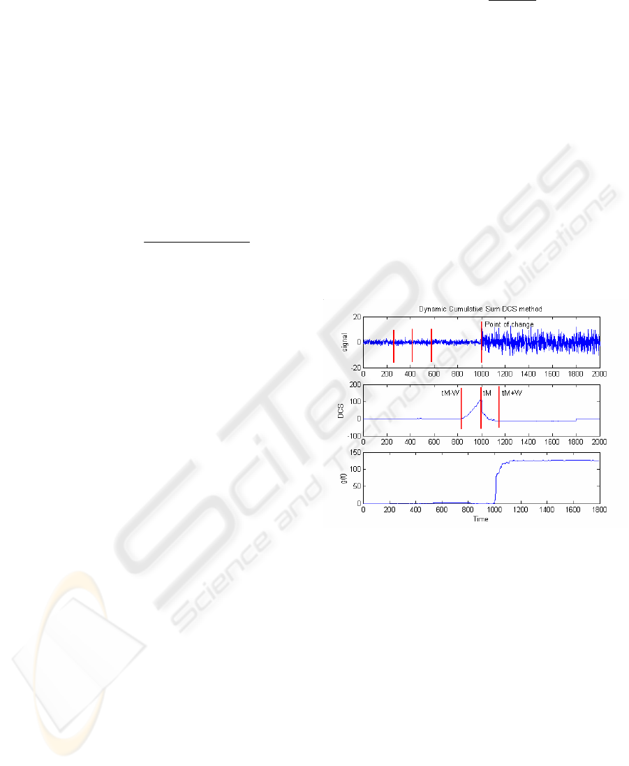
4.2 Dynamic Cumulative Sum Method
The Dynamic Cumulative Sum method (DCS) is
based on the local dynamic cumulative sum, around
the point of change t
r
, and can be used when the
parameters of the signal are unknown (
Khalil and
Duchêne, 2000). It is based on the local cumulative
sum of the likelihood ratios between two local
segments estimated at the current time t. These two
dynamic segments
)(t
a
S
(after t) and
)(t
b
S
(before t)
are estimated by using two windows of width W
(figure 2) before and after the instant t as follows:
•
}1,...,{i ;:
)(
−−= tWtxS
i
t
b
follows a
probability density function
()
i
xf
b
θ
•
},...,1{i ;:
)(
WttxS
i
t
a
++=
follows a
probability density function
()
i
xf
a
θ
The parameters
)(
^
t
b
θ
of the segment
)(t
b
S
, are
estimated using W points before the instant t and the
parameters
)(
^
t
a
θ
of the segment
)(t
a
S
, are estimated
using W points after the instant t. At a time t, and
for each level m, the DCS is defined as the sum of
the logarithm of likelihood ratios from the beginning
of the signal up to the time t:
∑∑
==
==
t
i
i
t
i
i
i
i
i
t
b
t
a
m
s
xf
xf
LnSSDCS
b
a
1
~
1
)(
)(
)(
)()(
)(
)(
),(
^
^
θ
θ
(4)
(Khalil, 1999) proves that the DCS function
reaches its maximum at the point of change t
r
. The
detection function used to estimate the point of
change is:
(
)
(
)
( ) ( ) () () ( ) () ()
1
max , ,
mmttmtt
t
ab ab
it
g
DCS S S DCS S S
≤≤
⎡⎤
=−
⎣⎦
(5)
The instant at which the procedure is stopped is t
s
= min {t : g
(m)
t
≥ h}, where h is the detection
threshold. The point of change is estimated as
follows:
t
c
= max {t>1 : g
(m)
t
= 0} (6)
Figure 2: Application of the DCS on a signal of abrupt
change. a) Original signal; b) DCS function; c) Detection
function g(t).
4.3 DCS Algorithm Combined with
MA-type Filters Bank
Decomposition
The detection is improved when the DCS method is
applied after ARMA or MA modeling, especially
when the signal presents no abrupt change, and the
direct application of the DCS algorithm leads to
ambiguous results that are sometimes difficult to
interpret for accurate fault detection. In case of MA
modeling, (i.e. a
i
= 0), equation (2) leads to (7):
∑
=
−=
p
i
mm
itxibty
0
)()(
)()()(
(7)
Θ
before
Θ
after
a
b
c
ICINCO 2008 - International Conference on Informatics in Control, Automation and Robotics
104

In (
Mustapha and al., 2007b), the detectability of
the DCS algorithm after MA – type filters bank is
proved. The basic idea is to prove that a change in a
parameter is equivalent to a change of the sign of the
expectation of the logarithm of the likelihood ratio:
before the instant of change,
0)(
~
>
t
SE
and after
instant of change
0)(
~
<
t
SE
where :
)]
)(
1
)(
1
(
)(
)(
[
2
1
)(
)(2)(2
2
)(2
)(2
~
t
b
t
a
t
t
b
t
a
t
t
xLnSLnS
σσσ
σ
−+==
(8)
and
)(
)(
t
a
σ
stands for the variance of the segment
)(t
a
S
and
)(
)(
t
b
σ
for the variance of the segment
)(t
b
S .
For MA filter and assuming that the successive
samples of x(t) are independent, (8) leads to (9):
[]
() 2
~
() 2
22 22
() 2 () 2
00
()
1
()
2
()
1111
() ( ) () ( ) )
22
() ()
t
a
t
t
t
b
nn
tt
ii
ab
ES ELnS E Ln
bixt i bixt i
γ
γ
γγ
==
⎡
⎡⎤
== +
⎢
⎢⎥
⎣⎦
⎣
⎤
−− −
⎥
⎦
∑∑
(9)
For t < t
r
- W,
)(t
a
S
and
)(t
b
S
are identical and have
the same characteristics so,
~
()0
t
ES =
. For t
r
- W < t
< t
r
,
)(t
a
S
and
)(t
b
S
are no longer identical and
0)(
~
>
t
SE
, and for t
r
< t < t
r
+ W we have
0)(
~
<
t
SE
.
Finally for t > t
r
+ W,
)(t
a
S
and
)(t
b
S
are identical
again and
~
()0
t
ES =
.
This demonstrates that
~
t
S
increases before t
r
, rea-
ches a maximum at t
r
then decreases. So, in order to
detect the point of change t
r
, we search to detect the
maximum of
~
t
S
by using the detection function g
t
.
5 FUSION TECHNIQUE
Because the detection algorithm is applied
individually to each frequency component, it is
important to apply a fusion technique to the resulting
times of change in order to get a single value for a
given fault in the system. The fusion technique is
achieved as follows:
-Each point of change at a given level is
considered as an interval [t
c
-a, t
c
+a], where a is
an arbitrary number of points taken before and
after the point of change.
-All the time intervals that have a common time
area are considered to correspond to the same
fault.
-The resulting point of change t
f
is calculated as
the center of gravity (or mean) of the
superimposed intervals.
6 APPLICATION TO TECP
In this section, the method, based on filters bank
decomposition and DCS algorithm, is applied to
detect disturbances on the Tennessee Eastman
Challenge Process (TECP; Downs and Vogel, 1993).
The TECP is a multivariable non-linear, high
dimensionality, unstable open-loop chemical reactor,
that is a simulation of a real chemical plant provided
by the Eastman company. There are 20 disturbances
IDV1 through IDV20 that could be simulated
(Downs and Vogel, 1993;
Singhal, 2000). The
sampling period for measurements is 60 seconds.
The TECP offers numerous opportunities for
control and fault detection and isolation studies. In
this work, we use a robust adaptive multivariable (4
inputs and 4 outputs) RTRL neural networks
controller (
Leclercq and al., 2005; Zerkaoui and al.,
2007) This controller compensates all perturbations
IDV1 to IDV 20 excepted IDV1, IDV6 and IDV7.
The figure 3 illustrates the advantage of our
method to detect changes for real world FDI
applications. Measurements of the reactor
temperature (figure 3a) are decomposed into 3
components and according a 3 – channels band pass
filters bank (figure 3c, d, e). The sampling frequency
of this signal is 0.0167 Hz and the normalized
central frequencies of the filters are: f
c1
= 0.64,
f
c2
= 0.74, f
c3
= 0.77. From time t
r
= 600 hours, the
unknown perturbation IDV16 modifies the dynamic
behavior of the system. The detection functions
applied on the 3 components (figure 3f, g, h) can be
compared with the detection function applied
directly on the measurement of pressure (figure 3b).
The detection results are considerably improved
by using the filters bank as a -preprocessing. In that
case, the DCS applied on original signal is not
suitable to detect the perturbation whereas the DCS
combined with 3- channels band pass filters bank
can detect the perturbation. After fusion, the
estimated instant of change is t
f
= 669 hours that
include a large delay to detection of 69 hours.
FAULT DETECTION BY MEANS OF DCS ALGORITHM COMBINED WITH FILTERS BANK - Application to the
Tennessee Eastman Challenge Process
105

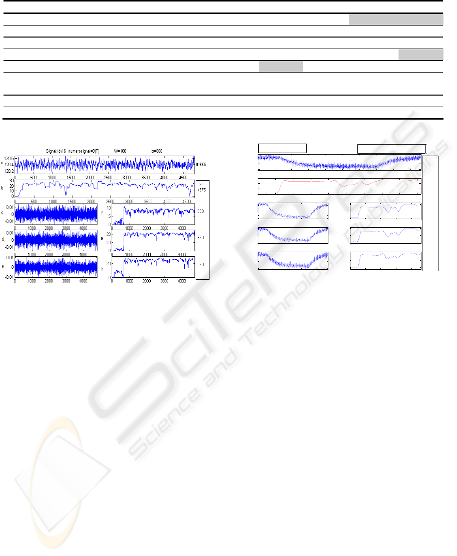
Table 1: Detection delays for several perturbations in TECP.
Disturbance Significance T° Pr sepL StrL
IDV 2 B composition, A/C ratio constant (step) 599/677 601/ 665 510/ 535 502/518
IDV 3 D feed temperature (step) 665/680 X X X
IDV 4 Reactor cooling water inlet temperature (step) 602/603 X X X
IDV 8 A, B, C feed composition (random variation) 650/660 650/660 513/634 343/353
IDV 9 D feed temperature (random variation) 279/287 X X X
IDV 11 Reactor cooling water inlet temperature (random
variation)
607/608 X X X
IDV 16 Unknown 647/670 X X X
IDV 17 Unknown 660/850 X X X
Figure 3: Analysis of the reactor temperature
measurements (°C) for TECP with robust adaptive control
and for IDV 16 perturbation from t
r
= 600. a) Original
signal b) DCS applied directly on the original signal
c) d) e)Decomposition using band pass filters(m = 1,2,3)
f) g) h) Detection functions applied on the filtered signals
(c, d, e).
The diagnosis of numerous perturbations has
been investigated with our method in order to show
the efficiency of the approach. All perturbations
have been simulated starting from time t
r
= 600
hours. The table 1 shows the results obtained with
various measured signals and various perturbations.
Two studies have been considered:
•
For perturbations IDV 2 – 3 – 4 – 8 – 9 – 11 –16
–17, the detection has been investigated in a
systematic way from the measurements of
temperature in reactor.
•
For perturbations IDV 2 and IDV 9, the
detection has been compared depending on the
measured variable (T, Pr, StrL, SepL).
0 500 1000 1500 2000 2500 3000 3500 4000 4500
40
45
50
a
Original signal
0 500 1000 1500 2000 2500 3000 3500 4000 4500
0
200
400
b
0 1000 2000 3000 4000
-4
-2
0
2
4
c
0 1000 2000 3000 4000
-5
0
5
d
0 1000 2000 3000 4000
-5
0
5
e
0 1000 2000 3000 4000
0
0.5
1
f
0 1000 2000 3000 4000
0
0.5
1
g
0 1000 2000 3000 4000
0
0.5
1
h
IDV2.mat ; numerosignal=12
W=200 ; tr=600
tc=
545
525
535
510
Figure 4: Analysis of the reactor separator level (%) for
TECP with robust adaptive control and for IDV 2
perturbation from t
r
= 600. a) Original signal b) DCS
applied directly on the original signal
c) d) e)Decomposition using band pass filters
(m = 1,2,3) f) g) h) Detection functions applied on the
filtered signals (c, d, e).
Table 1 shows the minimal and maximal values
of t
c
obtained over the three components. The
detection of changes was satisfactory in most cases
depending on the measured signals and the filters
that have been used. It is already important to notice
that IDV 2, that consists in a step in B composition,
cannot be detected with Y
3
and Y
4
(dark grey cells).
This perturbation corresponds to a modification of
the mean value that can be detected with other
methods (figure 4). IDV 8 and IDV 9 also present
some difficulties with some measured variable. But
an adaptation of threshold h used with detection
function and an adaptation of the central
decomposition frequencies will lead to acceptable
results. One can also notice the large dispersion of
the detection times in some cases.
tf=523
ICINCO 2008 - International Conference on Informatics in Control, Automation and Robotics
106

7 CONCLUSIONS
The aim of our work is to detect the point of change
of statistical parameters in signals issued from
complex industrial processes. This method uses a
band-pass filters bank combined with DCS to
characterize and classify the parameters of a signal
in order to detect any variation of the statistical
parameters due to any change in frequency and
energy. The proposed algorithm provides good
results for the detection of frequency changes in the
signal and can be used to detect the perturbation of
chemical processes as the TECP under stable closed
loop control. The results illustrate the interest of the
approach for on – line detection and real world
applications. Changes due to faults are easily
separated from changes due to input variations by
the comparative analysis of input and output
signals.
In the future, we will investigate detectability in
case of abrupt variations of the mean (figure 4). We
will also consider multiple faults investigation and
fault isolation based on signatures table of faults.
Fault isolation can be studied according to the
classification of the changes that are detected and
can certainly be improved by increasing the number
of considered filters and adapting their central
frequencies. We will also study the automatic
adaptation of the detection threshold h and complete
the diagnosis with faults identification.
REFERENCES
Basseville M., Nikiforov I. Detection of Abrupt Changes:
Theory and Application. Prentice-Hall, Englewood
Cliffs, NJ, 1993.
Blanke M., Kinnaert M., Lunze J., Staroswiecki M.,
Diagnosis and fault tolerant control, Springer Verlag,
New York, 2003.
Downs, J.J., Vogel, E.F, A plant-wide industrial control
problem, Computers and Chemical Engineering, 17,
pp. 245-255, 1993.
Falou W., "Une approche de la segmentation dans des
signaux de longue durée fortement bruités.
Application en ergonomie", PhD. Thesis, Université
de Technologie de Troyes, France, 2002.
Khalil M., Une approche pour la détection fondée sur une
somme cumulée dynamique associée à une
décomposition multiéchelle. Application à l'EMG
utérin. Dix-septième Colloque GRETSI sur le
traitement du signal et des images, Vannes,
France,1999.
M. Khalil, J. Duchêne. Uterine EMG Analyzing: A
dynamic approach for change detection and
classification. IEEE Transactions on Biomedical
Engineering, vol. 46, N6, pp. 748-756, juin 2000.
Leclercq, E., Druaux, F. Lefebvre, D., Zerkaoui, S.,
Autonomous learning algorithm for fully connected
recurrent networks. Neurocomputing, vol. 63, pp. 25-
44, 2005.
Mustapha O., Khalil M., Hoblos G, Chafouk H., Ziadeh
H., Lefebvre D., About the Detectability of DCS
Algorithm Combined with Filters Bank, Qualita 2007,
Tanger, Maroc, 2007.
Nikiforov I. Sequential detection of changes in stochastic
systems. Lecture notes in Control and information
Sciences, NY, USA, pp. 216-228, 1986.
Patton R.J., Frank P.M. and Clarck R., Issue of Fault
diagnosis for dynamic systems, Springer Verlag,
2000.
Singhal, A., Tennessee Eastman Plant Simulation with
Base Control System of McAvoy and Ye., Research
report, Department of Chemical Engineering,
University of California, Santa Barbara, USA, 2000.
Zerkaoui S., Druaux F., Leclercq E., Lefebvre D.,
Multivariable adaptive control for non-linear systems :
application to the Tennessee Eastman Challenge
Process, ECC 2007, Kos, Greece, 2007.
FAULT DETECTION BY MEANS OF DCS ALGORITHM COMBINED WITH FILTERS BANK - Application to the
Tennessee Eastman Challenge Process
107