PATH PLANNING USING DISCRETIZED EQUILIBRIUM PATHS
A Robotics Example
Cornel Sultan
Aerospace and Ocean Engineering Department, Virginia Tech, 215 Randolph Hall, Blacksburg, VA, U.S.A.
Keywords: Nonlinear control, equilibrium path, robot path planning.
Abstract: A collision avoidance path planning problem is considered and a simple solution which uses piecewise
constant controls generated by discretizing a feasible equilibrium path is presented and investigated.
1 INTRODUCTION
A new methodology has been recently proposed
(Sultan, 2007) for the control of nonlinear ODEs,
.,,
),,(
RTtRUuRXx
uxf
dt
dx
x
mn
⊂∈⊂∈⊂∈
==

(1)
Here f is a function of class C
k
in
UX ×
(k > 0), x,
u, and t are the state, control vectors, and time,
whereas X, U, and T are open sets in the n, m, and
one dimensional real spaces.
The key idea is to control (1) such that its state
space trajectory is close to an equilibrium path
obtained by solving
),(0 uxf= .
(2)
If
),(
ii
ux is a solution of (2) and
),(
iii
ux
x
f
J
∂
∂
=
is
not singular, there exist an open set U
e
and a unique
function g of class C
k
such that
.:g ,0)),((
),(),(
ee
ii
XUuugf
ugxugx
→=
==
(3)
Here U
e
is the largest domain in U in which (2) can
be solved uniquely for x as in (3) and
)),(( uug
x
f
∂
∂
is
not singular. If
),(
ff
ux
,
ef
Uu ∈
is a different
solution of (3),
i
u and
f
u
can be connected by a
curve
)(su
e
in
e
U , parameterized by
],0[
τ
∈s
,
feie
uuuu =
=
)(,)0(
τ
,
(4)
which is g-mapped onto an equilibrium path,
))(()( sugsx
ee
=
, ,)0(
ie
xx =
fe
xx =)(
τ
.
The control problem is to develop control laws
which guarantee that the state space trajectory of the
system is close to the equilibrium path, as illustrated
in Figure 1. In order to achieve this goal, the strategy
described next was proposed in (Sultan, 2007). The
controls are initially fixed at u
i
and when the
transition begins, at t=0, they start to vary along
e
u ,
)()( tutu
e
=
,
Tt ⊂
∈
],0[
τ
. When t reaches
τ
the
controls are frozen at the final, desired value:
⎪
⎩
⎪
⎨
⎧
>
≤≤
<
=
τ
τ
tu
ttu
tu
tu
f
e
i
,
0 ),(
0,
)(
.
(5)
The corresponding state space trajectory,
)(tx
d
,
called the deployment path, is the solution of
iddd
xxtuxfx =
=
)0()),(,(

.
(6)
If
)(
τ
d
x
belongs to the basin of attraction of
f
x
then the system’s trajectory will settle down,
asymptotically in time, to the desired final value,
f
x . Asymptotical stability of
f
x is crucial for the
application of this methodology.
236
Sultan C. (2008).
PATH PLANNING USING DISCRETIZED EQUILIBRIUM PATHS - A Robotics Example.
In Proceedings of the Fifth International Conference on Informatics in Control, Automation and Robotics - SPSMC, pages 236-239
DOI: 10.5220/0001480602360239
Copyright
c
 SciTePress

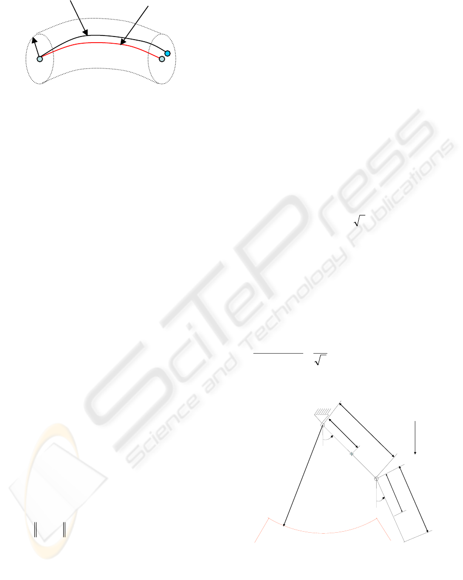
Figure 1: Deployment and equilibrium paths.
In this paper an example of a collision avoidance
path planning problem is considered. An equilibrium
path which satisfies the constraints is found and
discretized to generate piecewise constant controls
which are used to drive the system. It is important
to remark that this strategy is different from the one
proposed in (Sultan, 2007), where continuous
controls are used. Here, the parameterization of the
equilibrium path, originally continuous, is
discretized. One justification for this approach is the
easiness of discrete controls implementation.
2 THEORETICAL RESULTS
In the following two important results are given (the
proofs are omitted for brevity).
Theorem 1. If the equilibrium path is composed
only of asymptotically stable equilibria then, for
0>∀
ε
there exists a piecewise constant control
)(tu , obtained by discretizing the equilibrium path,
such that the distance between the corresponding
segments of the deployment and equilibrium paths is
less than
ε
(i.e. the deployment and equilibrium
paths are arbitrarily close).
Theorem 2. If the equilibrium path is composed
only of asymptotically stable equilibria and for any
u,
),( uxf is Taylor series expandable in x, for
0>∀
η
there exists a piecewise constant control
)(tu , obtained by discretizing the equilibrium path
such that
],0[,)( τη ∈∀< ttx
d

.
3 A PATH PLANNING PROBLEM
Consider a two link robotic manipulator in the
vertical plane (Figure 2). The links are rigid, the
system is placed in a constant gravitational field,
control torques and damping torques proportional to
the relative angular velocity between the moving
parts act at the joints. The equations of motion are:
111211
2
221212
1122121211
2
12
2
11
)sin()()sin(
)cos()(
uglmcmclm
dclmIlmcm
=++−
++−+++
θθθθ
θθθθθ


(7)
2222
2
121212
12222
2
22121212
)sin()sin(
)()()cos(
ugcmclm
dIcmclm
=+−
−−+++−
θθθθ
θθθθθθ


(8)
where angles
21
,
θ
θ
describe the motion, m
i
, l
i
, c
i
, I
i
,
are the mass, length, center of mass (CM) position,
transversal moment of inertia of the i-th link, d
i
and
u
i
are the damping coefficient and control torque at
joint i, respectively, g is the gravitational constant.
These equations can be easily cast into the first order
form (1). The numerical values (SI units) used are:
.81.9,5.0,12/
,5.0,3/1,5,10
21
212121
====
======
gddlmI
ccllmm
iii
(9)
The system must transition between two
equilibria,
0,70
21
==
ii
θθ
,
0,70
21
=−=
ff
θθ
.
Collision with a circular sector obstacle, of radius
R=1, described below, must be avoided:
.6030,60
300,0
3
1
)sin(
)30sin(
060,60
112
1
21
2
112
<≤−>
<<<−
−
−
≤<−+>
θθθ
θ
θθ
θ
θθθ
if
if
if
(10)
1
θ
2
θ
C
1
C
2
g
ˆ
R
l
1
l
2
Obstacle
CM
1
Figure 2: Two link robotic manipulator.
Equilibrium Path
Deployment Path
ε
x
f
x
i
PATH PLANNING USING DISCRETIZED EQUILIBRIUM PATHS - A Robotics Example
237

An equilibrium path which satisfies (10) is
].,[,cos62
111
11
1
2 fie
if
e
e
θθθ
θθ
θ
θ
∈
⎟
⎟
⎠
⎞
⎜
⎜
⎝
⎛
−
=
(11)
and the equilibrium controls are easily found,
).sin(
),sin()(
2222
112111
ee
ee
gcmu
lmcmgu
θ
θ
=
+=
(12)
The equilibrium path is parameterized using the
following class C
2
function
,0 ,)(
3
)(
630
)(
30
)(
2
345
11
5
11
τττ
θθ
τ
θθ
≤≤
⎟
⎟
⎠
⎞
⎜
⎜
⎝
⎛
−+−−
−+=
tt
t
t
tt
t
ifie
(13)
which is further discretized to obtain piecewise
constant controls using (11) and (12).
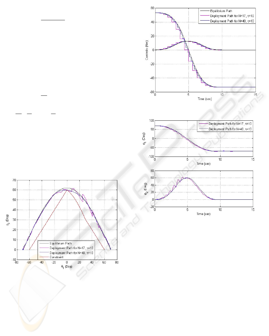
Consider
10=
τ
(“fast deployment”). Piecewise
constant controls are generated using N equal time
intervals. Figure 3 shows the deployment and
equilibrium paths.
Figure 3: Deployment paths for “fast” deployment.
Figures 4 and 5 give the time histories of the
controls and angles for N=17 and N=40. The
deployment error cannot be made small enough to
avoid the obstacle regardless of how large N is
(higher values of N were considered). Thus
τ
should be increased and the controls refined for the
deployment error to be sufficiently small.
Figure 4: Controls variation for “fast” deployment.
Figure 5: Generalized coordinates variation for “fast”
deployment.
In the second scenario, called “slow” deployment,
the deployment time is
20=
τ
and piecewise
constant controls are generated by discretizing (11-
13) with N=34 and N=80. Figures 8-10 show that
collision is avoided. The deployment error is smaller
because the deployment time is longer and finer
controls are used. It is important to mention that if
only the deployment time is increased the desired
result is not obtained; if N=17 or N=40 are used in
conjunction with
20
=
τ
, the deployment error is
still big and collision with the obstacle occurs.
ICINCO 2008 - International Conference on Informatics in Control, Automation and Robotics
238

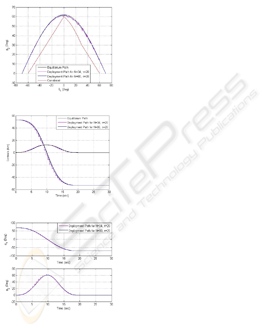
Figure 6: Deployment paths for “slow” deployment.
Figure 7: Controls variation for “slow” deployment.
Figure 8: Generalized coordinates variation for “slow”
deployment.
4 CONCLUSIONS
An example of a path planning problem is used to
illustrate the control of nonlinear systems using
equilibrium paths. The idea is to find an equilibrium
path which satisfies the collision avoidance
constraints, which is a much easier problem than
finding a dynamic path which satisfies the
constraints. Then the equilibrium path is discretized
to build piecewise constant controls which are used
to drive the system. Simulations indicate that for the
deployment and equilibrium paths to be close the
deployment time should be sufficiently long and the
controls sufficiently refined.
It is important to remark that the solution
investigated here uses discretizations of an
equilibrium path which satisfies the collision
avoidance constraints as opposed to continuous
parameterizations and hence continuous controls.
One justification for this approach is the easiness of
practical implementation of discrete controls.
REFERENCES
Sultan, C., 2007. Nonlinear systems control using
equilibrium paths. In Proceedings of the Conference
on Decision and Control, New Orleans, LA, USA.
PATH PLANNING USING DISCRETIZED EQUILIBRIUM PATHS - A Robotics Example
239