
EXPERIMENT
AL STUDY OF BOUNDING BOX ALGORITHMS
Darko Dimitrov
1
, Mathias Holst
2
, Christian Knauer
1
and Klaus Kriegel
1
1
Freie Universit
¨
at Berlin, Institute of Computer Science
Takustraße 9, D-14195 Berlin, Germany
2
Universit
¨
at Rostock, Institute of Computer Science
Albert Einstein Str. 21, D-18059 Rostock, Germany
Keywords:
Bounding Box Algorithms, Principal Component Analysis, Approximation Algorithms.
Abstract:
The computation of the minimum-volume bounding box of a point set in R
3
is a hard problem. The best known
exact algorithm requires O(n
3
) time, so several approximation algorithms and heuristics are preferred in prac-
tice. Among them, the algorithm based on PCA (Principal Component Analysis) plays an important role.
Recently, it has been shown that the discrete PCA algorithm may fail to approximate the minimum-volume
bounding box even for a large constant factor. Moreover, this happens only for some very special examples
with point clusters. As an alternative, it has been proven that the continuous version of PCA overcomes these
problems.
Here, we study the impact of the recent theoretical results on applications of several PCA variants in practice.
We give the closed form solutions for the case when the point set is a polyhedron or a polyhedral surface. To
the best of our knowledge, the continuous PCA over the volume of a 3D body is considered for the first time.
We analyze the advantages and disadvantages of the different variants on realistic inputs, randomly generated
inputs, and specially constructed (worst case) instances. The results reveal that for most of the realistic inputs
the qualities of the discrete PCA and the continuous PCA bounding boxes are comparable. As it was expected
the discrete PCA versions are much faster, but behave bad on the clustered inputs. In addition, we evaluate
and compare the performances of several existing bounding box algorithms.
1 INTRODUCTION
Many computer graphics algorithms use bounding
boxes, as containers of point sets or complex objects,
to improve their performance. For example, bounding
boxes are used to maintain hierarchical data structures
for fast rendering of a scene or for collision detection.
Moreover, there are applications in shape analysis and
shape simplification, or in statistics, for storing and
performing range-search queries on a large database
of samples.
A minimum-area bounding box of a set of n points in
R
2
can be computed in O(n logn) time, for example
with the rotating caliper algorithm (Toussaint, 1983).
(O’Rourke, 1985) presented a deterministic algo-
rithm, an elegant extension of the rotating caliper ap-
proach, for computing the minimum-volume bound-
ing box of a set of n points in R
3
. His algorithm re-
quires O(n
3
) time and O(n) space. Besides the high
run time, this algorithm is very difficult to implement,
and therefore, its main contributions are more of the-
oretical interest.
(Barequet and Har-Peled, 2001) have contributed two
(1+ε)-approximation algorithms for computing the
minimum-volume bounding box for point sets in R
3
,
both with nearly linear time complexity. The run-
ning times of their algorithms are O(n + 1/ε
4.5
) and
O(nlogn + n/ε
3
), respectively. Although the above
mentioned algorithms have guaranties on the quality
of the approximation and are asymptotically fast, the
constant of proportionality hidden in the O-notation is
quite big, which makes them unpractical. An excep-
tion is a simplified variant of the second algorithm of
Barequet and Har-Peled that is used in this study.
Numerous heuristics have been proposed for com-
puting a box which encloses a given set of points.
The simplest heuristic is naturally to compute the
axis-aligned bounding box of the point set. Two-
15
Dimitrov D., Holst M., Knauer C. and Kriegel K. (2008).
EXPERIMENTAL STUDY OF BOUNDING BOX ALGORITHMS.
In Proceedings of the Third International Conference on Computer Graphics Theory and Applications, pages 15-22
DOI: 10.5220/0001096600150022
Copyright
c
SciTePress

dimensional variants of this heuristic include the well-
known R-tree, the packed R-tree (Roussopoulos and
Leifker, 1985), the R
∗
-tree (Beckmann et al., 1990),
the R
+
-tree (Sellis et al., 1987), etc. Further heuristics
of computing tight fitting bounding boxes are based
on simulated annealing, or other optimization tech-
niques, for example Powell’s quadratic convergent
methods (Lahanas et al., 2000).
A frequently used heuristic for computing a
bounding box of a set of points is based on princi-
pal component analysis. The principal components
of the point set define the axes of the bounding box.
Once the axis directions are given, the spread of the
bounding box is easily found by the extreme values
of the projection of the points on the corresponding
axis. Two distinguished applications of this heuris-
tic are the OBB-tree (Gottschalk et al., 1996) and the
BOXTREE (Barequet et al., 1996). Both are hier-
archical bounding box structures which support effi-
cient collision detection and ray tracing. Computing a
bounding box of a set of points in R
2
and R
3
by PCA
is simple and requires linear time. The popularity of
this heuristic, besides its speed, lies in its easy im-
plementation and in the fact that usually PCA bound-
ing boxes are tight fitting. Recently, (Dimitrov et al.,
2007b) presented examples of discrete points sets in
the plane, showing that the worst case ratio of the vol-
ume of the PCA bounding box to the volume of the
minimum-volume bounding box tends to infinity (see
Figure 1 for an illustration in R
2
). It has been shown
in (Dimitrov et al., 2007a) that the continuous PCA
version on convex point sets in R
3
guarantees a con-
stant approximation factor for the volume of the re-
sulting bounding box. However, in many applications
this guarantee has to be paid with an extra O(n logn)
run time for computing the convex hull of the input
point set.
In this paper, we study the impact of the rather the-
oretical results above on applications of several PCA
variants in practice. We analyze the advantages and
disadvantages of the different variants on realistic in-
puts, randomly generated inputs, and specially con-
structed (worst case) instances. The main issues of
our experimental study can be subsumed as follows:
• The traditional discrete PCA algorithm works
very well on most realistic inputs. It gives a bad
approximation ratio on special inputs with point
clusters.
• The continuous PCA version can not be fooled by
point clusters. In practice, for realistic and ran-
domly generated inputs, it achieves much better
approximations than the guaranteed bounds. The
only weakness arises from symmetries in the in-
put.
• To improve the performances of the algorithms
we apply two approaches. First, we combine the
run time advantages of PCA with the quality ad-
vantages of continuous PCA by a sampling tech-
nique. Second, we introduce a postprocessing
step to overcome most of the problems with spe-
cially constructed outliers.
The paper is organized as follows: In Section 2,
we review the basics of the principal component anal-
ysis. We also consider the continuous version of PCA
and give the closed form solutions for the case when
the point set is a polyhedron or a polyhedral surface.
To the best of our knowledge, this is the first time that
the continuous PCA over the volume of the 3D body
has been considered. A few additional bounding box
algorithms and the experimental results are presented
in Section 3. The conclusion is given in Section 4.
2 PCA
The central idea and motivation of PCA (Jolliffe,
2002) (also known as the Karhunen-Loeve transform,
or the Hotelling transform) is to reduce the dimen-
sionality of a point set by identifying the most sig-
nificant directions (principal components). Let X =
{x
1
,x
2
,...,x
m
}, where x
i
is a d-dimensional vector,
and c = (c
1
,c
2
,...,c
d
) ∈ R
d
be the center of gravity
of X . For 1 ≤ k ≤ d, we use x
ik
to denote the k-th
coordinate of the vector x
i
. Given two vectors u and
v, we use hu,vi to denote their inner product. For any
unit vector v ∈ R
d
, the variance of X in direction v is
var(X,v) =
1
m
m
∑
i=1
hx
i
−c , vi
2
. (1)
The most significant direction corresponds to the unit
vector v
1
such that var(X, v
1
) is maximum. In gen-
eral, after identifying the j most significant directions
B
j
= {v
1
,...,v
j
}, the ( j + 1)-th most significant di-
rection corresponds to the unit vector v
j+1
such that
var(X,v
j+1
) is maximum among all unit vectors per-
pendicular to v
1
,v
2
,...,v
j
.
It can be verified that for any unit vector v ∈ R
d
,
var(X,v) = hCv, vi, (2)
where C is the covariance matrix of X. C is a sym-
metric d × d matrix where the (i, j)-th component,
c
i j
,1 ≤i, j ≤ d, is defined as
c
i j
=
1
m
m
∑
k=1
(x
ik
−c
i
)(x
jk
−c
j
). (3)
The procedure of finding the most significant direc-
tions, in the sense mentioned above, can be formu-
lated as an eigenvalue problem. If χ
1
> χ
2
> ···> χ
d
GRAPP 2008 - International Conference on Computer Graphics Theory and Applications
16
1stP C
2ndP C
1stP C
2ndP C
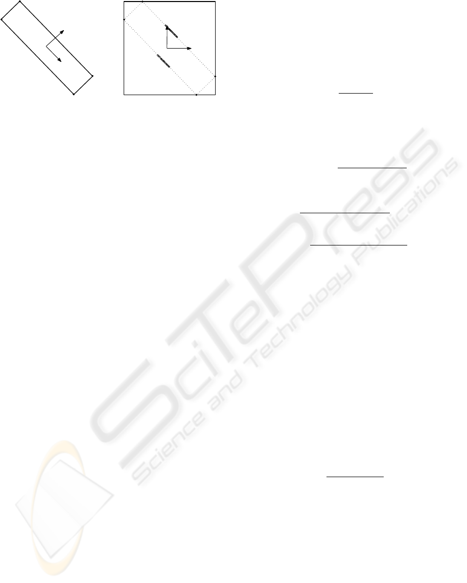
Figure 1: Four points and its PCA bounding-box (left).
Dense clusters of additional points significantly affect the
orientation of the PCA bounding-box (right).
are the eigenvalues of C, then the unit eigenvector
v
j
for χ
j
is the j-th most significant direction. All
χ
j
s are non-negative and χ
j
= var(X, v
j
). Since the
matrix C is symmetric positive definite, its eigenvec-
tors are orthogonal. If the eigenvalues are not dis-
tinct, the eigenvectors are not unique. In this case,
for eigenspaces of dimension bigger than 1, the or-
thonormal eigenvector basis is chosen arbitrary. How-
ever, distinct eigenvalues can be achieved by a slight
perturbation of the point set. Since bounding boxes
of a point set P (with respect to any given orthog-
onal coordinate system) depend only on the convex
hull CH(P), the construction of the covariance ma-
trix should be based only on CH(P) and not on the
distribution of the points inside. Using the vertices,
i.e., the 0-dimensional faces of CH(P) to define the
covariance matrix C a bounding box BB
pca(d,0)
(P) is
obtained. Let λ
d,0
(P) denote the approximation factor
for the given point set P ⊆R
d
and let
λ
d,0
= sup
n
λ
d,0
(P) | P ⊆ R
d
,Vol(CH(P)) > 0
o
the approximation factor in general. The example in
Figure 1 shows that λ
2,0
(P) can be arbitrarily large if
the convex hull is nearly a thin rectangle, with a lot of
additional vertices in the middle of the two long sides.
This construction can be lifted into higher dimensions
that gives a general lower bound, namely λ
d,0
= ∞
for any d ≥2. To overcome this problem, one can ap-
ply a continuous version of PCA taking into account
the dense set of all points on the boundary of CH(P),
or even all points in CH(P). In this approach X is a
continuous set of d-dimensional vectors and the coef-
ficients of the covariance matrix are defined by inte-
grals instead of finite sums. The computation of the
coefficients of the covariance matrix in the continuous
case can be done also in linear time, thus, the overall
complexity remains the same as in the discrete case.
2.1 Continuous PCA
Variants of the continuous PCA, applied on trian-
gulated surfaces of 3D objects, were presented by
(Gottschalk et al., 1996), (Lahanas et al., 2000) and
(Vrani
´
c et al., 2001). In what follows, we briefly re-
view the basics of the continuous PCA in a general
setting.
Let X be a continuous set of d-dimensional vec-
tors with constant density. Then, the center of gravity
of X is
c =
R
x∈X
xdx
R
x∈X
dx
. (4)
Here,
R
dx denotes either a line integral, an area inte-
gral, or a volume integral in higher dimensions. For
any unit vector v ∈ R
d
, the variance of X in direction
v is
var(X , v) =
R
x∈X
hx −c,vi
2
dx
R
x∈X
dx
. (5)
The covariance matrix of X has the form
C =
R
x∈X
(x −c)(x −c)
T
dx
R
x∈X
dx
, with (6)
c
i j
=
R
x
∈
X
(x
i
−c
i
)(x
j
−c
j
)dx
R
x∈X
dx
, (7)
where x
i
and x
j
are the i-th and j-th component of the
vector x, and c
i
and c
j
i-th and j-th component of the
center of gravity. The procedure of finding the most
significant directions, can be also reformulated as an
eigenvalue problem.
For point sets P in R
2
we are especially inter-
ested in the cases when X represents the boundary
of CH(P), or all points in CH(P). Since the first
case corresponds to the 1-dimensional faces of CH(P)
and the second case to the only 2-dimensional face of
CH(P), the generalization to a dimension d > 2 leads
to a series of d −1 continuous PCA versions. For a
point set P ∈ R
d
, C(P,i) denotes the covariance ma-
trix defined by the points on the i-dimensional faces
of CH(P), and BB
pca(d,i)
(P), denotes the correspond-
ing bounding box. The approximation factors λ
d,i
(P)
and λ
d,i
are defined as
λ
d,i
(P) =
Vol(BB
pca(d,i)
(P))
Vol(BB
opt
(P))
, and
λ
d,i
= sup
©
λ
d,i
(P) | P ⊆ R
d
,Vol(CH(P)) > 0
ª
.
In (Dimitrov et al., 2007b), it was shown that λ
d,i
=
∞ for any d ≥ 4 and any 1 ≤ i < d −1. This way,
there remain only two interesting cases for a given d:
the factor λ
d,d−1
corresponding to the boundary of the
convex hull, and the factor λ
d,d
corresponding to the
full convex hull.
The following lower and upper bounds on the
quality of the PCA bounding boxes were shown in
(Dimitrov et al., 2007a) and (Dimitrov et al., 2007b).
Theorem 2.1
• λ
3,2
≥ 4 and λ
3,3
≥ 4.
EXPERIMENTAL STUDY OF BOUNDING BOX ALGORITHMS
17

• If d is a power of two, then λ
d,d−1
≥
√
d
d
and
λ
d,d
≥
√
d
d
.
• λ
2,1
≤ 2.737.
• λ
2,2
≤ 2.104.
• λ
3,3
≤ 7.72.
The thorough tests on the realistic and synthetic
inputs revealed that the quality of the resulting bound-
ing boxes was better than the theoretically guaranteed
quality.
2.2 Evaluation of the Expressions for
Continuous PCA
Although the continuous PCA approach is based on
integrals, it is possible to reduce the formulas to ordi-
nary sums if the point set X is a polyhedron or a poly-
hedral surface. Due to space limitation, we present
here only the closed formulas for a convex polytope
and leave the polyhedral surface case and correspond-
ing cases in R
2
to the extended version of the paper.
Continuous PCA over a convex polytope. Let
X be a convex polytope in R
3
. We assume that the
boundary of X is triangulated (if it is not, we can
triangulate it in preprocessing). We choose an arbi-
trary point ~o in the interior of X , for example, we can
choose that ~o is the center of gravity of the bound-
ary of X. Each triangle from the boundary together
with ~o forms a tetrahedron. Let the number of such
formed tetrahedra be n. The i-th tetrahedron, with
vertices ~x
1,i
,~x
2,i
,~x
3,i
,~x
4,i
= ~o, can be represented in a
parametric form by
~
Q
i
(s,t,u) =~x
4,i
+ s (~x
1,i
−~x
4,i
) +
t (~x
2,i
−~x
4,i
) + u (~x
3,i
−~x
4,i
), for 0 ≤ s,t, u ≤ 1, and
s + t + u ≤1.
The center of gravity of the i-th tetrahedron is
~c
i
=
R
1
0
R
1−s
0
R
1−s−t
0
ρ(
~
T
i
(s,t))
~
Q
i
(s,t)dudt ds
R
1
0
R
1−s
0
R
1−s−t
0
ρ(
~
T
i
(s,t))dudt ds
,
where ρ(
~
T
i
(s,t)) is a mass density at a point
~
T
i
(s,t).
Since, we can assume ρ(
~
T
i
(s,t)) = 1, we have
~c
i
=
R
1
0
R
1−s
0
R
1−s−t
0
~
Q
i
(s,t)dudt ds
R
1
0
R
1−s
0
R
1−s−t
0
du dt ds
=
~x
1,i
+~x
2,i
+~x
3,i
+~x
4,i
4
.
The contributions of each tetrahedron to the center of
gravity of X is proportional to its volume. If M
i
is
the 3 ×3 matrix whose k-th row is ~x
k,i
−~x
4,i
, for k =
1...3, then the volume of the i-th tetrahedron is
v
i
= volume(Q
i
) =
|det(M
i
)|
3!
.
We introduce a weight to each tetrahedron that is pro-
portional with its volume, define as
w
i
=
v
i
∑
n
i=1
v
i
.
Then, the center of gravity of X is
~c =
n
∑
i=1
w
i
~c
i
.
The covariance matrix of the i-th tetrahedron is
C
i
=
R
1
0
R
1−s
0
R
1−s−t
0
(
~
Q
i
(s,t,u)−~c) (
~
Q
i
(s,t,u)−~c)
T
du dt ds
R
1
0
R
1−s
0
R
1−s−t
0
du dt ds
=
1
20
³
∑
4
j=1
∑
4
k=1
(~x
j,i
−~c)(~x
k,i
−~c)
T
+
∑
4
j=1
(~x
j,i
−~c)(~x
j,i
−~c)
T
´
.
The element C
ab
i
of C
i
, where a,b ∈{1, 2,3} is
C
ab
i
=
1
20
³
∑
4
j=1
∑
4
k=1
(x
a
j,i
−c
a
)(x
b
k,i
−c
b
)+
∑
4
j=1
(x
a
j,i
−c
a
)(x
b
j,i
−c
b
)
´
,
with ~c = (c
1
,c
2
,c
3
). Finally, the covariance matrix of
X is
C =
∑
n
i=1
w
i
C
i
.
We would like to note that the above expressions hold
also for a star-shape object, where ~o is the kernel of
the object.
3 EXPERIMENTAL RESULTS
We have implemented and integrated in our testing
environment a number of bounding box algorithms
for a point set in R
3
. The algorithms were imple-
mented using C++ and Qt, and tested on a Core Duo
2.33GHz with 2GB memory. Below we detail the al-
gorithms used in this study. The tests were performed
on real graphics models and synthetic data. The real
graphics models were taken from various publicly
available sources (Standford 3D scanning repository,
3D Cafe). The synthetic test data were obtained in
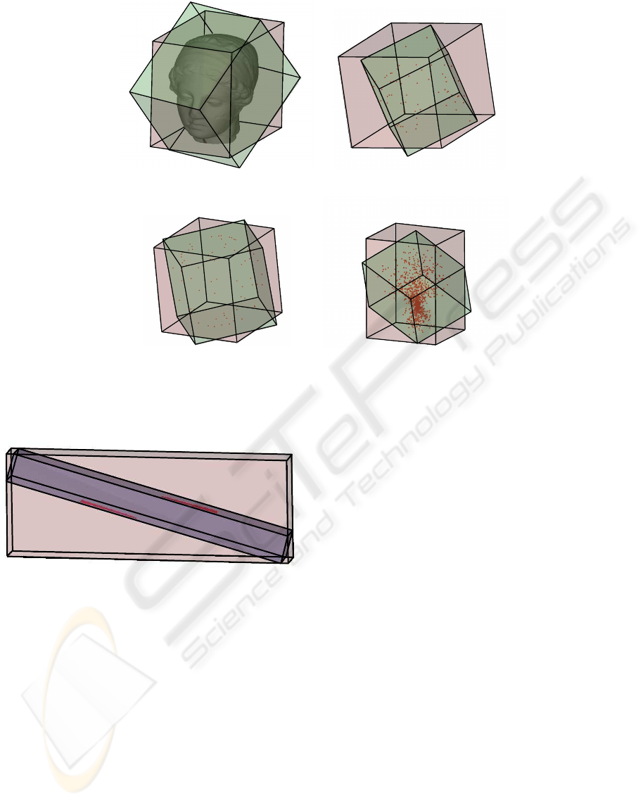
several manners (see Figure 2):
• uniformly generated point set on the unit sphere;
• randomly generated point set in the unit cube;
• randomly generated clustered point set in a box
with arbitrary spread.
To evaluate the influence of the clusters on the quality
of the bounding boxes obtained by discrete PCA, we
also generated clusters on the boundary of the real ob-
jects. The volume of a computed bounding box very
often can be ”locally” improved (decreased) by pro-
jecting the point set into a plane perpendicular to one
of the directions of the bounding box, followed by
computing a minimum-area bounding rectangle of the
projected set in that plane, and using this rectangle as
the base of an improving bounding box. This heuris-
tic converges to a local minimum. We encountered
GRAPP 2008 - International Conference on Computer Graphics Theory and Applications
18
a)
b)
c)
d)
Figure 2: Bounding boxes of four spatial point sets: a) real data (Igea model) b) randomly generated point set in the unit cube
c) uniformly generated point set on the unit sphere d) randomly generated clusters point set in a box with an arbitrary spread.
Figure 3: Extension of the example from Figure 1 in R
3
.
Dense collection of additional points (the red clusters) sig-
nificantly affect the orientation of the PCA bounding-box
of the cuboid. The outer box is the PCA bounding box, and
the inner box is the CPCA bounding box.
many examples when the reached local minimum was
not the global one. Each experiment was performed
twice, with and without this improving heuristic. The
parameter #iter in the tables below shows how many
times the computation of the minimum-area bounding
rectangle was performed to reach a local minimum.
3.1 Evaluation of the PCA and CPCA
Bounding Box Algorithms
We have implemented and tested the following PCA
and continuous PCA bounding box algorithms:
• PCA - computes the PCA bounding box of a dis-
crete point set.
• PCA-CH - computes the PCA bounding box of
the vertices of the convex hull of a point set.
• CPCA-area - computes the PCA bounding box of
a polyhedral surface.
• CPCA-area-CH - computes the PCA bounding
box of the boundary of the convex hull of an ob-
ject.
• CPCA-volume - computes the PCA bounding
box of a convex or a star-shaped object.
We have tested the above algorithms on a large
number of real and synthetic objects. Typical samples
of the results are given in Table 1 and Table 2. Due
to space limitations, we give more detailed results for
some of the tested data sets in the extended version
of the paper. For many of the tested data sets, the
volumes of the boxes obtained by CPCA algorithms
were slightly smaller than the volumes of the boxes
obtained by PCA, but usually the differences were
negligible. However, the CPCA methods have much
larger running times due to computing the convex
hull. Some of the synthetic data with clusters justifies
the theoretical results that favors the CPCA bounding
boxes over PCA bounding boxes. Figure 3 is a typi-
EXPERIMENTAL STUDY OF BOUNDING BOX ALGORITHMS
19
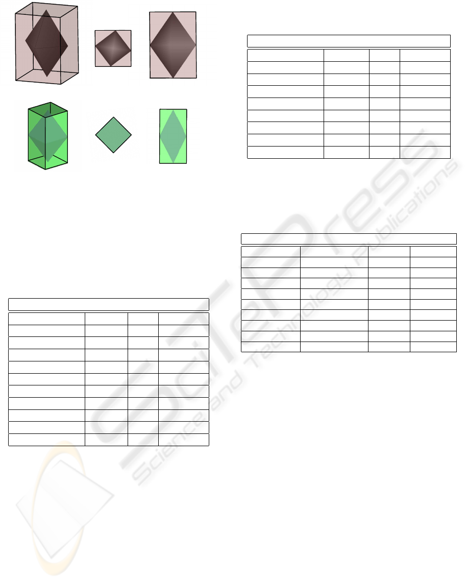
a)
b)
Figure 4: The dypiramid in the figure has two equal eigen-
values. a) The PCA bounding box and its top and side pro-
jections. b) The improved PCA bounding box and its top
and side projections.
cal example and indicates that the PCA bounding box
can be arbitrarily bad.
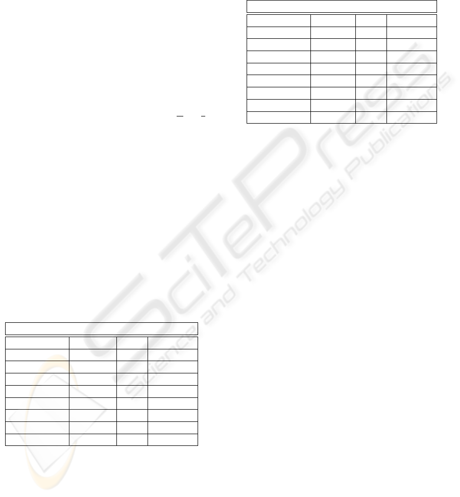
Table 1: Performance of the PCA bounding box algorithms
on a real data (Lucy: 262909 vertices, 525814 triangles, 622
convex hull vertices, 1240 convex hull triangles).
Lucy
algorithm volume #iter time[s]
PCA 756184 - 0.23635
improved 702004 2 2.90236
PCA-CH 736099 - 6.470
improved 704615 3 6.52645
CPCA-area 731496 - 0.533937
improved 692082 2 3.1634
CPCA-area-CH 726545 - 4.38215
improved 696356 2 4.47444
CPCA-volume 729131 - 5.31306
improved 699059 3 5.34954
As previously mentioned, for eigenspaces of dimen-
sion bigger than 1, the orthonormal basis of eigen-
vectors is chosen arbitrarily. This can result in un-
predictable and large bounding boxes, see Figure 4
for an illustration. We solve this problem by comput-
ing bounding boxes that are aligned with one principal
component. The other two directions are determined
by computing the exact minimum-area bounding rect-
angle of the projections of the points into a plane or-
thogonal to the first chosen direction.
If the input is given as a (triangulated) surface,
then we can improve the run time of the PCA and
PCA-area methods, without decreasing the quality of
the bounding boxes, by sampling the surface and ap-
plying the PCA on the sampled points. Once the
principal components are determined, we compute
Table 2: Performance of the PCA bounding box algorithms
on the clustered point set with 10000 points.
clustered point set
algorithm volume #iter time[s]
PCA 31.3084 - 0.036038
improved 17.4366 6 0.285556
PCA-CH 33.4428 - 1.93812
improved 17.4593 9 2.18226
CPCA-area-CH 21.0176 - 1.5961
improved 17.4559 3 1.66884
CPCA-volume 19.4125 - 1.32058
improved 17.4591 5 1.39327
Table 3: Performance of the sampling approach on a real
data (Igea: 134345 vertices, 268688 triangles). The values
in the table are the average of the results of 100 runs of
the algorithms, each time with a newly generated sampling
point set.
Igea
algorithm #sampling pnts volume time[s]
PCA - 6.73373 0.189644
PCA-area - 6.70684 0.297377
PCA-sample 50 6.81354 0.122567
PCA-sample 100 6.6936 0.123895
PCA-sample 1000 6.69176 0.131753
PCA-sample 10000 6.70855 0.13825
PCA-sample 50000 6.70546 0.178306
PCA-sample 60000 6.70629 0.173158
PCA-sample 70000 6.70525 0.188299
the bounding box of the original surface. We do the
sampling uniformly, in the sense that the number of
the sampled points on the particular triangle is pro-
portional to the relative area of the triangle. Table
3 shows the performance of this sampling approach
(denoted by PCA-sample) on a real model. The re-
sults reveal that even for a small number of sampling
points, the resulting bounding boxes are comparable
with the PCA and CPCA-area bounding boxes. Also,
if the number of the sampling points is smaller than
half of the original point set the sampling approach is
faster than PCA approach.
3.2 Evaluation of other Bounding Box
Algorithms
Next, we describe a few additional bounding box al-
gorithms, whose performance we have analyzed.
• AABB - computes the axis parallel bounding box
of the input point set. This algorithm reads the
points only once and as such is a good reference
in comparing the running times of the other algo-
rithms.
GRAPP 2008 - International Conference on Computer Graphics Theory and Applications
20
• BHP - this algorithm is based on the (1 +
ε)-approximation algorithm from (Barequet and
Har-Peled, 2001), with run time complexity
O(nlog n + n/ε
3
). It is an exhaustive grid-base
search, and gives by far the best results among
all the algorithms. In many cases, that we were
able to verified, it outputs bounding boxes that are
the minimum-volume or close to the minimum-
volume bounding boxes. However, due to the ex-
haustive search it is also the slowest one.
• BHP-CH - same as BHP, but on the convex hull
vertices.
• DiameterBB - computes a bounding box based
on the diameter of the point set. First, (1 −ε) - ap-
proximation of the diameter of P that determines
the longest side of the bounding box is computed.
This can be done efficiently in O(n +
1
ε
3
log
1
ε
)
time. See (Har-Peled, 2001) for more details. The
diameter of the projection of P onto the plain or-
thogonal to longest side of the bounding box de-
termines the second side of the bounding box. The
third side is determined by the direction orthogo-
nal to the first two sides. This idea is old, and can
be traced back to (Macbeath, 1951).
Note that DiameterBB applied on convex hull ver-
tices gives the same bounding box as applied on the
original point set.
Typical samples of the results are given in Table 4
and Table 5. Due to space limitation, we present more
results in the extended version of the paper.
Table 4: Performance of the additional bounding box algo-
rithms on a real data.
Lucy
algorithm volume #iter time[s]
AABB 789279 - 0.016606
improved 705152 3 4.92674
BHP 743677 - 3.25255
improved 705648 1 5.91975
BHP-CH 687723 - 8.63365
improved 687695 1 8.72115
DiameterBB 1504660 - 0.123361
improved 790190 4 4.89671
An improvement for a convex-hull method requires
less additional time than an improvement for a non-
convex-hull method. This is due to the fact that the
convex hull of a point set P in general has less than
|P| vertices. Once the convex hull in R
3
is computed,
it suffices to project it to the plane of projection to ob-
tain the convex hull in R
2
. It should be observed that
the number of iterations needed for the improvement
of the AABB method, as well as its initial quality, de-
pends heavily on the orientation of the point set.
Table 5: Performance of the additional bounding box algo-
rithms on the clustered point set with 10000 points. The
results were obtained on the same point set as those from
Table 2.
clustered point set
algorithm volume #iter time[s]
AABB 30.2574 - 0.000624
improved 16.4563 7 0.247101
BHP 15.5662 - 3.13794
improved 15.5662 0 3.13794
BHP-CH 15.5662 - 3.13335
improved 15.5662 0 3.13345
DiameterBB 31.5521 - 0.013173
improved 16.6952 4 0.205163
4 CONCLUSIONS
In short, we can draw the following conclusions:
• The traditional discrete PCA algorithm can be
easily fooled by inputs with point clusters. In con-
trast, the continuous PCA variants are not sensi-
tive to the clustered inputs.
• The continuous PCA version on convex point sets
guarantees a constant approximation factor for the
volume of the resulting bounding box. However,
in many applications this guarantee has to be paid
with an extra O(n logn) run time for computing
the convex hull of the input instance. The tests on
the realistic and synthetic inputs revealed that the
quality of the resulting bounding boxes was better
than the theoretically guaranteed quality.
• For most of the real world inputs the qualities of
the discrete PCA and the continuous PCA bound-
ing boxes are comparable.
• The run time of the discrete PCA and continu-
ous PCA (CPCA-area) heuristics can be improved
without decreasing the quality of the resulting
bounding boxes by sampling the surface and ap-
plying the discrete PCA on the sampled points.
This approach assumes that an input is given as a
(triangulated) surface. If this is not a case, a sur-
face reconstruction must be performed, which is
usually slower than the computation of the con-
vex hull.
• Both the discrete and the continuous PCA are sen-
sitive to symmetries in the input.
EXPERIMENTAL STUDY OF BOUNDING BOX ALGORITHMS
21

• The diameter based heuristic is not sensitive to
clusters and can be used as an alternative to con-
tinuous PCA approaches.
• An improvement step, performed by computing
the minimum-area bounding rectangle of the pro-
jected point set, is a powerful technique that of-
ten significantly decreases the existing bounding
boxes. This technique can be also used by PCA
approaches when the eigenvectors are not unique.
• The experiments show that the sizes of the bound-
ing boxes obtained by CPCA-area and CPCA-
volume are comparable. This indicates that the
upper bound of λ
3,2
, that is an open problem,
should be similar to that of λ
3,3
.
Future work includes obtaining closed form so-
lutions for the continuous PCA over non-polyhedral
objects. A practical and fast (1 + ε)-approximation
algorithm for the minimum-volume bounding box of
a point set in R
3
is also of general interest.
REFERENCES
Barequet, G., Chazelle, B., Guibas, L. J., Mitchell, J. S. B.,
and Tal, A. (1996). Boxtree: A hierarchical represen-
tation for surfaces in 3D. Computer Graphics Forum,
15:387–396.
Barequet, G. and Har-Peled, S. (2001). Efficiently approxi-
mating the minimum-volume bounding box of a point
set in three dimensions. J. Algorithms, 38(1):91–109.
Beckmann, N., Kriegel, H.-P., Schneider, R., and Seeger, B.
(1990). The R
∗
-tree: An efficient and robust access
method for points and rectangles. ACM SIGMOD Int.
Conf. on Manag. of Data, pages 322–331.
Dimitrov, D., Knauer, C., Kriegel, K., and Rote, G. (2007a).
New upper bounds on the quality of the PCA bound-
ing boxes in R
2
and R
3
. In Proc. 23rd Annu. ACM
Sympos. on Comput. Geom., pages 275–283.
Dimitrov, D., Knauer, C., Kriegel, K., and Rote, G. (2007b).
Upper and lower bounds on the quality of the PCA
bounding boxes. In Proc. 15th WSCG, pages 185–
192.
Gottschalk, S., Lin, M. C., and Manocha, D. (1996). OBB-
Tree: A hierarchical structure for rapid interference
detection. In SIGGRAPH 1996, pages 171–180.
Har-Peled, S. (2001). A practical approach for computing
the diameter of a point-set. In Proc. 17th Annu. ACM
Sympos. on Comput. Geom., pages 177–186.
Jolliffe, I. (2002). Principal Component Analysis. Springer-
Verlag, New York, 2nd ed.
Lahanas, M., Kemmerer, T., Milickovic, N., K. Karouzakis,
D. B., and Zamboglou, N. (2000). Optimized bound-
ing boxes for three-dimensional treatment planning in
brachytherapy. In Med. Phys. 27, pages 2333–2342.
Macbeath, A. M. (1951). A compactness theorem for affine
equivalence classes of convex regions. Canadian J.
Math., 3:54–61.
O’Rourke, J. (1985). Finding minimal enclosing boxes. In
Int. J. Comp. Info. Sci. 14, pages 183–199.
Roussopoulos, N. and Leifker, D. (1985). Direct spatial
search on pictorial databases using packed R-trees. In
ACM SIGMOD, pages 17–31.
Sellis, T., Roussopoulos, N., and Faloutsos, C. (1987). The
R
+
-tree: A dynamic index for multidimensional ob-
jects. In 13th VLDB Conference, pages 507–518.
Toussaint, G. (1983). Solving geometric problems with
the rotating calipers. In IEEE MELECON, pages
A10.02/1–4.
Vrani
´
c, D. V., Saupe, D., and Richter, J. (2001). Tools for
3D-object retrieval: Karhunen-Loeve transform and
spherical harmonics. In IEEE 2001 Workshop Mul-
timedia Signal Processing, pages 293–298.
GRAPP 2008 - International Conference on Computer Graphics Theory and Applications
22
