CONTINUOUS

LEARNING OF SIMPLE VISUAL CONCEPTS USING

INCREMENTAL KERNEL DENSITY ESTIMATION

∗

Danijel Sko

caj, Matej Kristan and Ale

s Leonardis

Faculty of Computer and Information Science, University of Ljubljana Tr

zaˇska 25, SI-1001 Ljubljana, Slovenia

Keywords:

Continuous learning, incremental learning, incremental kernel density estimation, learning associations.

Abstract:

In this paper we propose a method for continuous learning of simple visual concepts. The method continu-

ously associates words describing observed scenes with automatically extracted visual features. Since in our

setting every sample is labelled with multiple concept labels, and there are no negative examples, reconstruc-

tive representations of the incoming data are used. The associated features are modelled with kernel density

probability distribution estimates, which are built incrementally. The proposed approach is applied to the

learning of object properties and spatial relations.

1 INTRODUCTION

An important characteristic of a system that operates

in a real-life environment is the ability to expand its

current knowledge. The system has to create and ex-

tend concepts by observing the environment – and

has to do so continuously, in a life-long manner. An

integral part of such a continuous learning system

is a method for incremental updating of previously

learned representations, which has to fulﬁll several

requirements: (i) the learning algorithm should be

able to update the current representations (and create

new ones if necessary), (ii) it should not require ac-

cess to old (previously processed) original data, (iii)

the representations should be kept compact, and (iv)

the computational effort needed for a single update

should not depend on the amount of previously ob-

served data.

In this paper we present an algorithm that ad-

dresses these requirements in the context of learn-

ing associations between low-level visual features and

higher-level concepts. In particular, we address the

problem of continuous learning of visual properties

(such as colour or shape) and spatial relations (such

as ‘to the left of’ or ‘far away’). The main goal is

to ﬁnd associations between words describing these

concepts and simple visual features extracted from

∗

This

research has been supported in part by the

EU project CoSy (FP6-004250-IP) and Research program

Computer Vision P2-0214 (RS).

images.

In our setting, the inputs in the learning process

are partial descriptions of the scene; descriptions of

the objects and relationships between them. An ob-

ject can be labeled with several concept labels (e.g.,

object A can be ‘yellow’ and ‘round’ and positioned

‘in the middle’ of the image and ‘to the left of’ object

B). These descriptions serve as learning examples.

There are no negative examples (e.g., the information

that ‘yellow’ is not ‘red’ is not provided). Therefore,

the algorithm should build reconstructive representa-

tions without relying on discriminative information,

which would discriminate between different classes

(i.e., concepts) (Fidler et al., 2006). It can only ex-

ploit consistency of the feature values extracted from

the objects labelled with the same concept and speci-

ﬁcity of these values with respect to the rest of the

feature values related to other concept labels.

The contribution of this paper is twofold. First, we

present a method that is able to continuously process

input feature vectors and learn corresponding associa-

tions based on the consistency and speciﬁcity criteria.

Similar problems are commonly referred to as exam-

ples of the symbol grounding problem and have of-

ten been tackled by different researchers in different

settings (Harnad, 1992; Ardizzone et al., 1992; Roy

and Pentland, 2002; Roy, 2002; Vogt, 2002). Sev-

eral papers have also been published addressing on-

line learning, particularly with regard to object recog-

nition (Kirstein et al., 2005; Steels and Kaplan, 2001;

Arsenio, 2004). In our system, however, we utilize,

598

Sko

caj D., Kristan M. and Leonardis A. (2008).

CONTINUOUS LEARNING OF SIMPLE VISUAL CONCEPTS USING INCREMENTAL KERNEL DENSITY ESTIMATION.

In Proceedings of the Third International Conference on Computer Vision Theory and Applications, pages 598-604

 SciTePress

in a uniﬁed framework, continuous online learning of

qualitative object properties and spatial relations in

a setting with no negative examples and when every

sample is labelled with multiple concept labels, with

a view toward using this as a basis for further learning

and facilitating unlearning as well.

To facilitate this type of learning, our method

models the values of features, that are associated

with individual concepts, by estimating the probabil-

ity density function that generated them. To that end,

we employ kernel density estimates (KDE), which

apply a mixture of kernels to approximate the un-

derlying density. Since the models have to be esti-

mated continuously from the arriving data, we con-

struct a kernel for each incoming data and use it to

update the corresponding distributions. This boils

down to estimating the single parameter of the kernel

– its bandwidth. We propose a method for estimat-

ing the bandwidth of each incoming kernel, which

is the second contribution of this paper. A number

of bandwidth selection methods have been proposed

previously which aim to minimize the asymptotic-

mean-integrated-squared-error (AMISE) between the

unknown original distribution and its approximation

based on a set of the observed samples (e.g., Wand

and Jones (Wand and Jones, 1995)). However, these

approaches are not directly applicable in incremental

settings. To that end, various incremental approaches

have been proposed which usually incorporate some

constraints or prior knowledge of the relation between

the consecutive samples (Elgammal et al., 2002; Han

et al., 2004), like temporal coherence on the incom-

ing data (Arandjelovic and Cipolla, 2005; Song and

Wang, 2005). Szewczyk (Szewczyk, 2005) applies a

Dirichlet process prior on components and applies a

Gamma density prior to sample the bandwidth of the

incoming data. A drawback of this approach, how-

ever, is that the parameters of the prior need to be

speciﬁed for a given problem. Here, we propose an

incremental bandwidth selection approach that does

not assume any temporal coherence and does not re-

quire setting a large number of parameters.

The paper is organised as follows. First we intro-

duce the main incremental learning algorithm. Then

we explain the algorithm for incremental updating of

KDE representations. In section 4 we then present

the evaluation of the proposed methods. Finally, we

summarize and outline some work in progress.

2 MAIN INCREMENTAL

LEARNING ALGORITHM

The main task of the incremental algorithm is to as-

sign associations between extracted visual features

and the corresponding visual concepts. Since our

system is based on positive examples only (we do

not have negative examples for the concepts being

learned), and each input instance can be labelled with

several concept labels, the algorithm can not exploit

discriminative information and can rely only on re-

constructive representations of observed visual fea-

tures. Each visual concept is associated with a vi-

sual feature that best models the corresponding im-

ages according to the consistency and speciﬁcity cri-

teria. It must determine which of the automatically

extracted visual features are consistent over all im-

ages representing the same visual concept and that

are, at the same time, speciﬁc for that visual concept

only. The learning algorithm thus selects from a set

of one-dimensional features (e.g., median hue value,

area of segmented region, coordinates of the object

center, distance between two objects, etc.), the feature

whose values are most consistent and speciﬁc over all

images representing the same visual concept (e.g., all

images of large objects, or circular objects, or pairs of

objects far apart etc.). Note that this process should

be performed incrementally, considering only the cur-

rent image (or a very recent set of images) and learned

representations – previously processed images cannot

be re-analysed.

Therefore, at any given time, each concept is asso-

ciated with one visual feature, i.e., with the represen-

tation built from previously observed values of this

feature. A Kernel Density Estimate (KDE) is used

to model the underlying distribution that generated

these values. The KDE models, in our case Gaussian

mixture models, are updated at every step by consid-

ering the current model and new samples using the

algorithm presented in the next section. However, af-

ter new samples have been observed, it may turn out

that some other feature would better ﬁt the particu-

lar concept. The system enables such switching be-

tween different features by keeping simpliﬁed repre-

sentations of all features. Assuming that the data that

has to be modeled is coarsely normally distributed the

proposed algorithm keeps updating the Gaussian rep-

resentations of all features for every concept being

learned

. These updates can be performed without

loss of information. When at some point the algo-

rithm determines that some other feature is to be asso-

ciated with the particular concept, it starts building a

In practice, only the representations of a number of po-

tentially interesting features could be maintained.

CONTINUOUS LEARNING OF SIMPLE VISUAL CONCEPTS USING INCREMENTAL KERNEL DENSITY

ESTIMATION

599

new KDE, starting with one component obtained from

the corresponding Gaussian model

The only question that still remains is how to

select the best feature. The algorithm fulﬁlls the

consistency and speciﬁcity criteria mentioned above

by selecting the feature with a distribution that is

most distant from the distributions of the correspond-

ing feature values of all other concepts. The dis-

tances between two distributions are measured us-

ing the Hellinger distance [16]. Note that while the

Hellinger distance can be calculated exactly for two

Gaussians, there is no closed-form solution for Gaus-

sian mixtures. We therefore apply the unscented-

transform (Julier and Uhlmann, 2005) to approxi-

mate the Hellinger distance between two mixtures.

The proposed incremental learning algorithm is pre-

sented

in Algorithm 1.

The learned concepts are than used for analysis

of new images. Feature vectors are extracted from

the image and evaluated with a recognition algorithm

that for every concept returns a belief, a value in the

range from 0 to 1. This value is obtained by verifying

how well the value of the feature, which is assigned

to the concept, ﬁts the particular KDE distribution,

i.e., p

(i)

= getBelief(mC

(i)

.KDE, f

(mC

(i)

). This esti-

mation can be done in different ways; our algorithm

returns the integral over the pdf values that have lower

probability than the current sample.

3 INCREMENTAL ESTIMATION

OF KDE

In the previous section we described the main algo-

rithm for incremental learning of simple visual con-

cepts. Since these concepts are described using ker-

nel density estimates (in our case mixtures of one-

dimensional Gaussians), we present here an approach

to incremental construction of these estimates.

Formally we deﬁne a Gaussian-kernel-based

KDE as an M-component mixture of Gaussians

p(x) =

∑

j=1

(x−x

), (2)

In practice, several KDEs of the most interesting fea-

tures could be maintained.

The following notation is used: mC

(i)

represent nc

models of concepts being learned, where mC

(i)

( j)

is a

Gaussian model of the j-th feature and mC

(i)

.KDE is a KDE

model of the best feature (mC

(i)

.B) for the i-th concept. f

is a n f −dimensional training feature vector, c is a list of

the corresponding concept labels. The subscripts t −1 and

t indicate the time step.

Algorithm 1 Main incremental learning algorithm.

Input: mC

(i)

t−1

;i = 1...nc

t−1

, f

, c

// current models

and current input

Output: mC

(i)

,i = 1... nc

// updated models

// Update Gaussian models

for i ∈ c

do // for all current concept labels

if i /∈mC

t−1

then // previously unencountered

concept

= nc

t−1

+ 1 // increase the number of

concepts

init(mC

(i)

) // initialize a new concept

else // existing concept

for j = 1.. . nf do // for all features

(i)

( j)

= updateG(mC

(i)

t−1

( j)

, f

( j)

)

// update Gaussian models

end for

end if

end for

// Select best features

for i = 1...nc

do // for all learned concepts

for j = 1.. . nf do // for all features

i j

∑

k=1

Hel

(pd f 1, pd f 2),

where // calculate Hellinger

distances

pd f 1 =

(

(i)

.KDE , if mC

(i)

.B = j

(i)

( j)

, if mC

(i)

.B 6= j

(1)

pd f 2 =

(

(k)

.KDE , if mC

(k)

.B = j

(k)

( j)

, if mC

(k)

.B 6= j

end for

(i)

.B = argmax

// determine the best feature

end for

// Update KDE models

for i = 1...nc

do // for all learned concepts

if mC

(i)

.B 6= mC

(i)

t−1

.B then // new best feature

(i)

.KDE = mC

(i)

(mC

(i)

.B)

// initialize

KDE with corresp. Gaussian

else // still the same best feature

if i ∈ c

then // current concept label

(i)

.KDE =

updateKDE(mC

(i)

t−1

.KDE, f

(mC

(i)

.B)

)

using Algorithm 2

else // not current concept label

(i)

.KDE = mC

(i)

t−1

.KDE // keep the old

model

end if

end for

VISAPP 2008 - International Conference on Computer Vision Theory and Applications

600

where w

is the weight of the j-th component and

(x−µ) is a Gaussian kernel

(z) = (2πσ

)

−1

exp(−

/σ

), (3)

centered at mean µ with standard deviation σ; note

that σ is also known as the bandwidth of the kernel.

Suppose that we observe a set of n

samples {x

}

i=1:n

up to the current time-step t. We seek a kernel density

estimate with kernels of equal bandwidths h

ˆp

(x;h

) =

∑

i=1

(x−x

), (4)

which is as close as possible to the underlying distri-

bution that generated the samples. A classical mea-

sure used to deﬁne closeness of the estimator ˆp

(x;h

)

to the underlying distribution p(x) is the mean inte-

grated squared error (MISE)

MISE = E[ ˆp

(x;h

) −p(x)]

. (5)

Applying a Taylor expansion, assuming a large

sample-set and noting that the kernels in ˆp

(x;h

)

are Gaussians ((Wand and Jones, 1995), p.19), we

can write the asymptotic MISE (AMISE) between

ˆp

(x;h

) and p

(x) as

AMISE =

√

)

−1

R(p

(x)), (6)

where p

(x) is the second derivative of p(x) and

R(p

(x)) =

(x)

dx. Minimizing AMISE w.r.t.

bandwidth h

gives AMISE-optimal bandwidth

tAMISE

= [

√

πR(p

(x))n

]

. (7)

Note that (7) cannot be calculated exactly since it

depends on the second derivative of p(x), and p(x)

is exactly the unknown distribution we are trying to

approximate. Several approaches to approximating

R(p

(x)) have been proposed in the literature (see e.g.

(Wand and Jones, 1995)), however these require ac-

cess to all observed samples, which forgoes the pos-

sibility of incremental learning where we wish to dis-

card previous samples and retain only compact rep-

resentations of them. Thus in our setting we have to

estimate the bandwidth of the kernel corresponding to

the incoming sample and update the existing density

estimate using that kernel; we propose a plug-in rule

to achieve that.

Let x

be the currently observed sample and let

ˆp

t−1

(x) be an approximation to the underlying distri-

bution p(x) from the previous time-step. Note that

in incremental learning we compress the estimated

distributions once in a while to maintain low com-

plexity (Leonardis and Bischof, 2005). Therefore,

in general, the bandwidths of the kernels in ˆp

t−1

(x)

may vary. The current estimate of p(x) is initial-

ized using the distribution from the previous time-

step ˆp

(x) ≈ ˆp

t−1

(x). The bandwidth

of the ker-

nel K

(x−x

) corresponding to the current observed

sample x

is obtained by approximating the unknown

distribution p(x) ≈ ˆp

(x) and applying (7)

= c

scale

√

πR( ˆp

(x))n

]

−1/5

, (8)

where c

scale

is used to increase the bandwidth a lit-

tle and thus avoid undersmoothing. In our experi-

ence, values of the scale parameter c

scale

∈ [1, 1.5] in

(8) give reasonable results and in all our experiments

scale

= 1.3 is used. The resulting kernel K

(x −x

)

is then combined with ˆp

t−1

(x) into an improved esti-

mate of the unknown distribution

ˆp

(x) = (1 −

) ˆp

t−1

(x) +

(x−x

). (9)

Next, the improved estimate ˆp

(x) from (9) is plugged

back in the equation (8) to re-approximate

and thus

equations (8) and (9) are iterated until convergence;

usually, ﬁve iterations sufﬁce. The entire procedure is

outlined in Algorithm 2.

Algorithm 2 Incremental density approximation algo-

rithm.

Input: ˆp

t−1

(x), x

... the current density approxima-

tion and the new sample

Output: ˆp

(x) ... the new approximation of density

1: Initialize the estimate of the current distribution

ˆp

(x) ≈ ˆp

t−1

(x).

2: Estimate the bandwidth h

of K

(x −x

) accord-

ing to (8) using ˆp

(x).

3: Reestimate ˆp

(x) according to (9) using K

(x −

4: Iterate steps 2 and 3 until convergence.

5: If the number of components in ˆp

(x) exceeds a

threshold N

comp

, compress ˆp

(x).

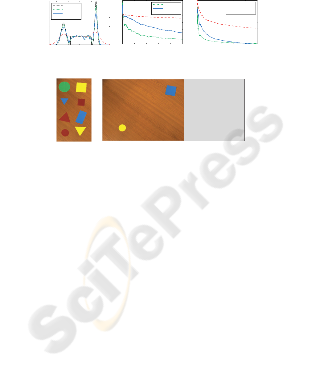
4 EXPERIMENTAL RESULTS

In this section we present two sets of experiments,

which were conducted to evaluate the proposed meth-

ods. The aim of the ﬁrst experiment was to demon-

strate the incremental bandwidth selection method

proposed in Section 3. We generated 1000 samples

from a 1D mixture of Gaussians and a uniform dis-

tribution (Figure 1(a)). These samples were then

used one at a time to incrementally build the ap-

proximation to the original distribution using Algo-

rithm 2. At each time-step two other KDE approxi-

mations were also built for reference: an optimal and

CONTINUOUS LEARNING OF SIMPLE VISUAL CONCEPTS USING INCREMENTAL KERNEL DENSITY

ESTIMATION

601

−1 −0.5 0 0.5 1

0.5

1.5

200 400 600 800

0.1

0.2

0.3

0.4

0.5

0.6

error

Number of samples

200 400 600 800

0.05

0.1

0.15

0.2

0.25

0.3

0.35

bandwidth

Number of samples

Source

Optimal

Our method

Silverman

Optimal

Our method

Silverman

Optimal

Our method

Silverman

(a) (b) (c)

Figure 1: Illustration of Incremental KDE algorithm: (a) ﬁnal estimated distributions, (b) MISE with respect to the source

distribution, (c) estimated bandwidth.

A is yellow, small, and circular.

B is blue, large, and square.

A is on the left.

A is near.

B is on the right.

B is far away.

A is to the left of B.

A is closer than B.

A is far from B.

B is to the right of A.

B is further away than A.

B is far from A.

(a) (b)

Figure 2: (a) Input shapes. (b) Training / automatically generated scene description.

a suboptimal. These were batch approximations, and

were thus built by processing all samples observed

up to the given time-step simultaneously. The op-

timal bandwidth was estimated using the solve-the-

equation plug-in method (Jones et. al, 1996), which

is currently theoretically and empirically one of the

most successful bandwidth selection methods. For the

suboptimal bandwidth selection we have chosen Sil-

verman’s rule-of-thumb ((Wand and Jones, 1995), pg.

60), which was also used to initialize our algorithm

from the ﬁrst two samples.

The results are shown in Figure 1. The ﬁnal

KDEs, after observing all 1000 samples, estimated by

the proposed incremental method and the two refer-

ence methods, are shown in Figure 1(a). It is clear

that Silverman produced an undersmoothed approx-

imation to the ground-truth distribution. The incre-

mentally constructed KDE and the batch-estimated

KDE using the solve-the-equation plug-in both visu-

ally agree well with the ground-truth. This can be

further quantitatively veriﬁed from Figure 1(b) where

we show how the integrated squared error (ISE) be-

tween the three approximations and the ground-truth

was changing as new samples were observed. While

initially errors are high for all three approximations

they decrease as new samples arrive. As expected,

the error of the KDE calculated using Silverman’s

rule remains high even after all 1000 samples have

been observed. On the other hand, the error de-

creases faster for the KDE constructed by the pro-

posed method and comes close to the error of the

optimally selected bandwidth with increasing num-

bers of samples. Note that the optimal bandwidth

was calculated using all samples observed up to a

given step. On the other hand, the proposed incremen-

tal method produced similar bandwidths using only a

low-dimensional representation of the observed sam-

ples (Fig.1(c)).

We evaluated the proposed method for learning

visual concepts in a task that involved learning

concepts of several object properties and spatial

relations using simple objects of basic shapes and of

different colours and sizes (Fig. 2(a)). This image

domain is quite suitable for such analysis, since the

object properties are very diverse and well deﬁned.

The input images contained pairs of objects that

were placed on a table in different conﬁgurations.

For every object, we considered ten visual concepts

related to the object’s colour, size and shape (red,

green, blue, yellow; small, large; square, circular,

triangular, and rectangular). Next, we also consid-

ered eleven different spatial relations – six binary

relations between the two objects (with respect to

the observer/camera): ‘to the left of’, ‘to the right

of’, ‘closer than’, ‘further away than’, ‘near to’,

‘far from’, and ﬁve unary relations describing the

position of the object in the scene: ‘on the left’, ‘in

the middle’, ‘on the right’, ‘near’, and ‘far away’.

Fig. 2(b) depicts one image with the corresponding

description, which gave two training samples (for

object A and object B). From every training sample

11 features were extracted (three appearance features,

VISAPP 2008 - International Conference on Computer Vision Theory and Applications

602

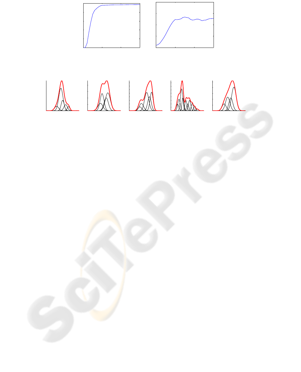
0 50 100 150

100

no of added samples

accuracy

0 50 100 150

no of added samples

average number of components

(a) (b)

Figure 3: Experimental results: (a) accuracy. (b) average number of components.

0.32 0.33 0.34 0.35 0.36 0.37

350 400 450 500 550 600

x 10

−3

−1000 −500 0 500

x 10

−4

0 100 200 300 400

x 10

−3

600 700 800 900 1000 1100

x 10

−3

Figure 4: Final models for ‘green’, ‘large’, ‘to the left of’, ‘on the left’, and ‘on the right’.

three shape features, and ﬁve distance features),

which were to be associated with 21 visual concepts

being learned.

We randomly divided a set of 300 samples into

two halves consisting of training and test samples

respectively. Then we added training samples one by

one and at each step updated the models of object

properties and spatial relations using the proposed

method. We evaluated the current models by trying

to recognize all training samples and observing the

achieved accuracy. To limit the complexity of the

models, the current KDE was compressed whenever

the number of components exceeded the number 20.

The experiment was repeated 20 times with dif-

ferent sequences of input samples. The average re-

sults are depicted in Fig. 3. From Fig. 3(a) it can be

seen that the overall accuracy increases by adding new

samples. The growth of the accuracy is very rapid at

the beginning when new models of newly introduced

concepts are being added, but still remains positive

even after all models are formed due to reﬁnement

of the corresponding associations and representations.

Fig. 3(b) plots the average number of Gaussian com-

ponents in KDE distributions of all models. One can

observe that after a while this number does not grow

any more, thus the model size remains limited. The

models do not improve by increasing their complex-

ity, but rather due to reﬁnement of the underlying rep-

resentations. Fig. 4 depicts kernel density estimates of

their best features for ﬁve concepts at the end of the

learning process. These trained models can be used

for automatic generation of scene descriptions as pre-

sented in Fig. 2(b).

5 CONCLUSIONS

In this paper we proposed a method for continuous

learning of simple visual concepts and applied it to

learning object properties and spatial relations. The

method keeps continuously establishing associations

between automatically extracted visual features and

words describing the observed scenes. The associated

features are modelled with kernel density probability

distribution estimates using the proposed incremental

KDE algorithm.

The proposed method fulﬁlls four requirements

for incremental learning presented in the introduction:

(i) the learning algorithm is able to update the current

representations and create new ones when new con-

cepts occur, (ii) it does not require access to old data

(it uses only their representations), (iii) the represen-

tations are kept compact and do not grow any more

once they reach an adequate complexity, and, con-

sequently (iv) the computational effort needed for a

single update at a given time does not depend on the

amount of data observed up until that time.

The work presented in this paper is a part of a

larger framework for continuous learning of concepts

that we have been developing. We will embed this

algorithm in an interactive setting, where the concept

labels (descriptions of scenes) will be obtained in an

interactive dialogue with the tutor. In this way nega-

tive training examples will also be introduced, which

will enable correction of erroneous updates. The pro-

posed algorithm was tailored to support such opera-

tions. In addition we also plan to extend the proposed

incremental KDE algorithm to multiple dimensions

and to advance the method to handle associations with

CONTINUOUS LEARNING OF SIMPLE VISUAL CONCEPTS USING INCREMENTAL KERNEL DENSITY

ESTIMATION

603

several features, as well as to improve the feature se-

lection method. Our ultimate goal is to develop a gen-

eral, scalable and robust method for continuous learn-

ing of visual concepts.

REFERENCES

Fidler, S., Sko

caj, D., Leonardis, A., Combining re-

constructive and discriminative subspace methods for

robust classiﬁcation and regression by subsampling.

IEEE Transactions on Pattern Analysis and Machine

Intelligence 28 (2006) 337–350

Harnad, S., The symbol grounding problem. Physica D:

Nonlinear Phenomena 42 (1990) 335–346

Ardizzone, E., Chella, A., Frixione, M., Gaglio, S., Inte-

grating subsymbolic and symbolic processing in artiﬁ-

cial vision. Journal of Intelligent Systems 1(4) (1992)

273–308

Roy, D.K., Pentland, A.P., Learning words from sights and

sounds: a computational model. Cognitive Science 26

(2002) 113–146

Roy, D.K., Learning visually-grounded words and syntax

for a scene description task. Computer Speech and

Language 16(3) (2002) 353–385

Vogt, P., The physical symbol grounding problem. Cogni-

tive Systems Research 3 (2002) 429–457

Kirstein, S., Wersing, H., K

orner, E., Rapid online learn-

ing of objects in a biologically motivated recognition

architecture. In: 27th DAGM. (2005) 301–308

Steels, L., Kaplan, F., AIBO’s ﬁrst words. the social learn-

ing of language and meaning. Evolution of Commu-

nication 4 (2001) 3–32

Arsenio, A., Developmental learning on a humanoid robot.

In: IEEE International Joint Conference On Neural

Networks. (2004) 3167–3172

Wand, M.P., Jones, M.C., Kernel Smoothing. Chapman &

Hall/CRC (1995)

Elgammal, A., Duraiswami, R., Harwood, D., Davis, L.,

Background and foreground modeling using nonpara-

metric kernel density estimation for visual surveil-

lance. In: Proceedings of the IEEE. (2002) 1151–

1163

Han, B., Comaniciu, D., Davis, L., Sequential density ap-

proximation through mode propagation: Applications

to background modeling. In: Asian Conf. Computer

Vision. (2004)

Arandjelovic, O., Cipolla, R., Incremental learning of

temporally-coherent gaussian mixture models. In:

British Machine Vision Conference. (2005) 759–768

Song, M., Wang, H., Highly efﬁcient incremental estima-

tion of gaussian mixture models for online data stream

clustering. In: SPIE: Intelligent Computing: Theory

and Applications. (2005) 174–183

Szewczyk, W.F., Time-evolving adaptive mixtures. Techni-

cal report, National Security Agency (2005)

Julier, S., Uhlmann, J., A general method for approximating

nonlinear transformations of probability distributions.

Technical report, Department of Engineering Science,

University of Oxford (1996)

Leonardis, A., Bischof, H., An efﬁcient MDL-based

construction of RBF networks. Neural Networks

11(1998) 963 – 973

Jones, M.C., Marron, J.S., Sheather, S.J., A brief survey of

bandwidth selection for density estimation. J. Amer.

Stat. Assoc. 91 (1996) 401–407

VISAPP 2008 - International Conference on Computer Vision Theory and Applications

604