ESTIMATING VEHICLE VELOCITY USING RECTIFIED IMAGES

Cristina Maduro, Katherine Batista, Paulo Peixoto and Jorge Batista

∗

ISR-Institute of Systems and Robotics, Department of Electrical Engineering, FCTUC

University of Coimbra, Coimbra, Portugal

Keywords:

Image rectiﬁcation, vehicle velocity, video sequences.

Abstract:

In this paper we propose a technique to estimate vehicles velocity, using rectiﬁed images that represent a top

view of the highway. To rectify image sequences captured by uncalibrated cameras, this method automatically

estimates two vanishing points using lines from the image plane. This approach requires two known lengths

on the ground plane and can be applied to highways that are fairly straight near the surveillance camera. Once

the background image is rectiﬁed it is possible to locate the stripes and boundaries of the highway lanes. This

process may also be used to count vehicles, estimate their velocities and the mean velocity associated to each

of the previously identiﬁed highway lanes.

1 INTRODUCTION

The incessant advances in camera technology along

with the constant improvement in areas such as com-

puter vision have lead to the development of auto-

matic and robust methods to estimate vehicle velocity.

However, this task is problematic when the image se-

quences do not preserve length ratios and parallelism

between lines. This difﬁculty can be easily solved by

the creation and employment of virtual images which

preserve the referred characteristics, acknowledged as

rectiﬁed images. These rectiﬁed images by repre-

senting a ”top view” of the observed scenario, sim-

plify the task of estimating velocity in trafﬁc surveil-

lance systems. This process demands the estimation

of two vanishing points using lines from the image

plane. Nevertheless, it is important to state that this

procedure is constrained to the precision with which

the required vanishing points are estimated. Thus, a

robust RANSAC (Fischler and Bolles, 1981) based

algorithm is applied in the estimation of the neces-

sary vanishing points. These are necessary to calcu-

late the homogeneous representation of the vanishing

line. This vanishing line is used in the calculation

of the projective transformation that rectiﬁes the im-

age sequence. Once attained the required projective

transformation it is then possible to rectify video se-

quences, and therefore estimate vehicle velocity and

extract lane topology. The highway lane boundaries

∗

This work was supported by BRISA, Auto-estradas de

Portugal, S.A.

can be easily located once identiﬁed the position of

the striped lines on the rectiﬁed background image.

Seeing as the striped lines follow a periodic distribu-

tion, these can be located by applying the autocor-

relation function to each line of the rectiﬁed back-

ground image. In order to estimate vehicle veloc-

ity, a Kalman ﬁlter (Kalman and Bucy, 1960) based

tracking system is employed to infer future vehicle

positions given a sequence of images. The estimation

of an object’s displacement or motion using informa-

tion extracted from two consecutive images can be

obtained using Lucas-Kanade’s optical ﬂow method

(Lucas and Kanade, 1981). Nonetheless, we chose to

employ a Kalman ﬁlter to correct the estimation pro-

vided by the previously referred method. Given the

fact that the output of this procedure is represented

in pixels per frame it is necessary to estimate a scale

factor that relates distances on the ground plane with

distances on the image plane. Once obtained the re-

quired scale factor and known the video’s framerate,

this procedure presents the object’s velocity in the de-

sired units. This paper is organized in four main sec-

tions. The ﬁrst, named Image Rectiﬁcation, focuses

on the method that originates the required rectiﬁed

images. The second section is referent to the pro-

cedure applied to estimate the necessary scale factor,

while the third section presents the process that esti-

mates vehicle velocity. To conclude, several results,

such as, rectiﬁed images and data referent to velocity

estimation are presented.

551

Maduro C., Batista K., Peixoto P. and Batista J. (2008).

ESTIMATING VEHICLE VELOCITY USING RECTIFIED IMAGES.

In Proceedings of the Third International Conference on Computer Vision Theory and Applications, pages 551-558

DOI: 10.5220/0001088205510558

 SciTePress

2 IMAGE RECTIFICATION

The perspective transformation associated to image

formation, distorts certain geometric properties, such

as length, angle and area ratios. Due to this fact, the

employment of video or image sequences in trafﬁc

surveillance is challenging, in particular for the task

of vehicle velocity estimation. However, this prob-

lem can be solved by using rectiﬁed images that re-

store the lost geometric properties to the images of

the monotorized scenario. A rectiﬁed image can be

attained by estimating a homographic transformation.

This estimation could be acquired by using the intrin-

sic and extrinsic camera parameters. Unfortunately,

the surveillance cameras are uncalibrated and there-

fore, these parameters are unknown. Consequently,

several methods have been developedin order to auto-

matically restore geometric propertiesto objects mov-

ing on a ground plane. Namely, D. Dailey (Dailey and

Cathey, 2005) presents a method that estimates the lo-

cation of one vanishing point in order to calibrate the

surveillance camera and achieve the required images.

However, this method presupposes the knowledge of

one of the angles of orientation of the surveillance

camera, and therefore cannot be applied to all surveil-

lance systems. On the other hand, in (Schoepﬂin

and Dailey, 2003), associated with T. Schoepﬂin, D.

Dailey presents a method that requires the estimation

of two vanishing points from lines that are parallel

and orthogonal to the road. This method estimates

the camera orientation and focal length, though the

height at which it is located is not automatically es-

timated. L. Grammatikopoulos, G. E. Karras and E.

Petsa in (Lazaros Grammatikopoulos, 2002), present

a method to measure vehicle speed using rectiﬁed im-

ages. This approach determines one vanishing point

and requires the knowledge of one known length one

the ground plane. Nevertheless, this method does not

rectify images from cameras that aren’t aligned ac-

cordingly to an axis parallel to the direction of mo-

tion. On the other hand, B. Bose and E. Grimson in

(Bose and Grimson, 2003), present a method similar

to the method employed in this study. The method

proposed by Bose and Grimson achieves metric rec-

tiﬁcation of the ground plane by tracking two objects

that travel with constant and possibly unequal speed.

In this paper, a method presented by D. Liebowitz

and A. Zisserman (Liebowitz and Zisserman, 1998) is

successfully employed in the rectiﬁcation of images.

This technique requires the estimation of two van-

ishing points and the prior knowledge of two angles

on the ground plane. Given the nature of a roadway

structure, i.e. the large amount of parallel and perpen-

dicular lines, these parameters can be easily obtained.

In a general manner, this method estimates the pro-

jective transformation by establishing three matrices

or transformations.

H = H

(1)

where H

represents the similarity transformation,

the afﬁne and H

the pure projective transforma-

tion. Each one of these transformations is responsible

for the reinstatement of certain geometric and met-

ric properties and can be achieved using known pa-

rameters on the image and ground planes. Namely,

the pure projective transformation is responsible for

restoring line parallelism and area ratios to the sce-

nario. This transformation can be easily acquired

by estimating the homogeneous representation of the

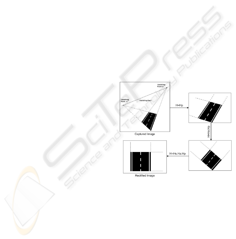
vanishing line. Once known the location of two van-

ishing points, this representation is quite straightfor-

ward, as can be seen in the following equation:

l =





= v

x v

(2)

where l is the homogeneous representation of the

vanishing line and v

and v

the vanishing points that

are represented on the upper left box in Figure 1.

Figure 1: Stages of the rectiﬁcation process.

Therefore, the pure projective transformation can

be represented by the following matrix:





1 0 0

0 1 0





(3)

where H

represents the referred pure projective

transformation. Hence, a correct estimation of this

transformation relies on the accurateness of the loca-

tion of the vanishing points. These are obtained by

applying the Hough transform to edges extracted from

the imaged highway lanes and to edges identiﬁed on

the foreground image.

VISAPP 2008 - International Conference on Computer Vision Theory and Applications

552

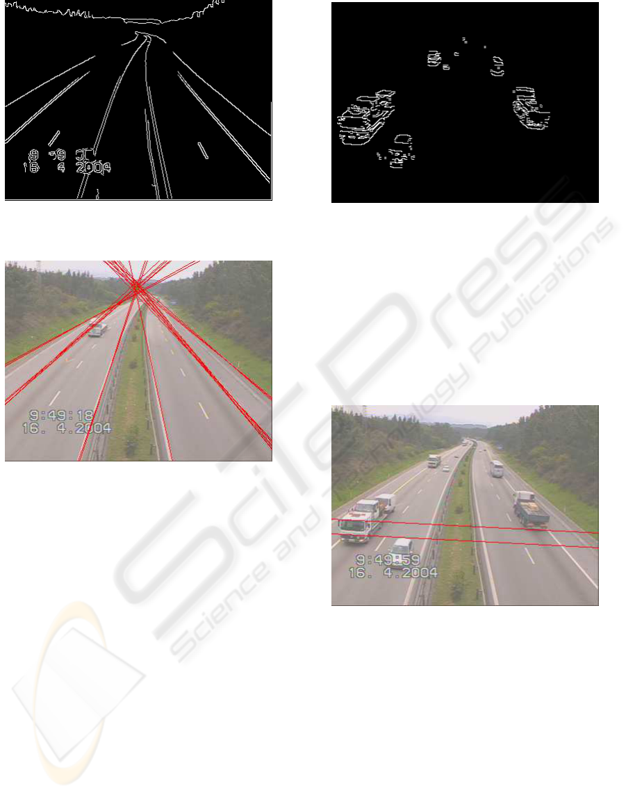
Figure 2: Edges detected by applying the Canny Edge De-

tector to the Background image.

Figure 3: Lines identiﬁed using the edges represented in

Figure 2.

Figure 2 represents an example of the edges de-

tected from a background image, while Figure 3 il-

lustrates the lines extracted from the previous image.

However, edges detected from the background image

may contain unnecessary edges. Due to this fact, an

activity map is estimated. An activity map is an im-

age that represents the regions that contain movement

throughout the image sequence, i.e. the regions of in-

terest. By applying an AND operator to the image

shown on Figure 2 and to the activity map, results an

image that contains only the sought edges. By def-

inition a vanishing point is the intersection point of

lines on the image plane that represent parallel lines

on the ground plane. Nevertheless, given the fact that

these lines do not intersect on an exact point, the van-

ishing point is situated on the point whose distance is

minimal to each one of these lines. Therefore, one of

the required vanishing points is obtained applying the

least squares method.

To determine the second vanishing point it is nec-

essary to identify edges that are predominately hori-

zontal on the foreground image. This image can be

Figure 4: Edges detected by applying the Canny Edge De-

tector to the Background image.

attained by subtracting each frame to the background

image and shows segmented vehicles. Figure 4 illus-

trates edges detected from the foreground, i.e. seg-

mented vehicles, using Sobel Detector that identiﬁes

horizontal edges. The lines represented in Figure 5

where obtained from the edges represented in Figure4

and are only a few of the used in the calculation of the

second vanishing point.

Figure 5: Lines identiﬁed using the edges represented in

Figure 4.

Given the fact that a great amount of lines ob-

tained from the foreground image are outliers, the es-

timation of this vanishing point using the least squares

method is erroneous. Thus, a RANSAC based algo-

rithm is used in this estimation. However, it is impor-

tant to state that the employed RANSAC algorithm

must contemplate the fact that the vanishing point

might be situated at inﬁnity. In order to do so, it is

necessary to adopt a 3D homogeneous representation

for the extracted lines. This form of representation

takes into account points at inﬁnity. Each iteration

of the RANSAC algorithm estimates a possible van-

ishing point using equation (4). The vanishing point

with the largest number of inliers is taken as the cor-

ESTIMATING VEHICLE VELOCITY USING RECTIFIED IMAGES

553

rect vanishing point.

p = l

x l

, (4)

where l

and l

represent the homogeneous coordi-

nates of two lines. The accuracy of this estimation is

crucial, and seeing as this algorithm is highly robust,

though computationally heavy, it presents ﬁne results

in the estimation of the required vanishing point.

On the other hand, the afﬁne transformation rein-

states angle and length ratios of non parallel lines,

and can be obtained using two known angles on the

ground plane as explained in (Liebowitz and Zisser-

man, 1998). This approach estimates two parame-

ters α and β using constraints on the ground plane.

These parameters represent the coordinates of the cir-

cular points on the afﬁne plane. Liebowitz and Zis-

serman in (Liebowitz and Zisserman, 1998) propose

three types of constraints:

• A known angle on the ground plane;

• equality of two unknown angles;

• a known length ratio.

Given the orthogonal structure of the highway lanes,

we chose to employ the ﬁrst constraint in this algo-

rithm, i.e. a known angle on the ground plane. Each

known angle on the ground planes deﬁnes a constraint

circle. This fact is quite useful seeing as α and β lie

within this circle represented on a complex space de-

ﬁned by (α,β). Therefore, in order to obtain the re-

quired parameters one may estimate the intersection

of two constraint circles obtained using two different

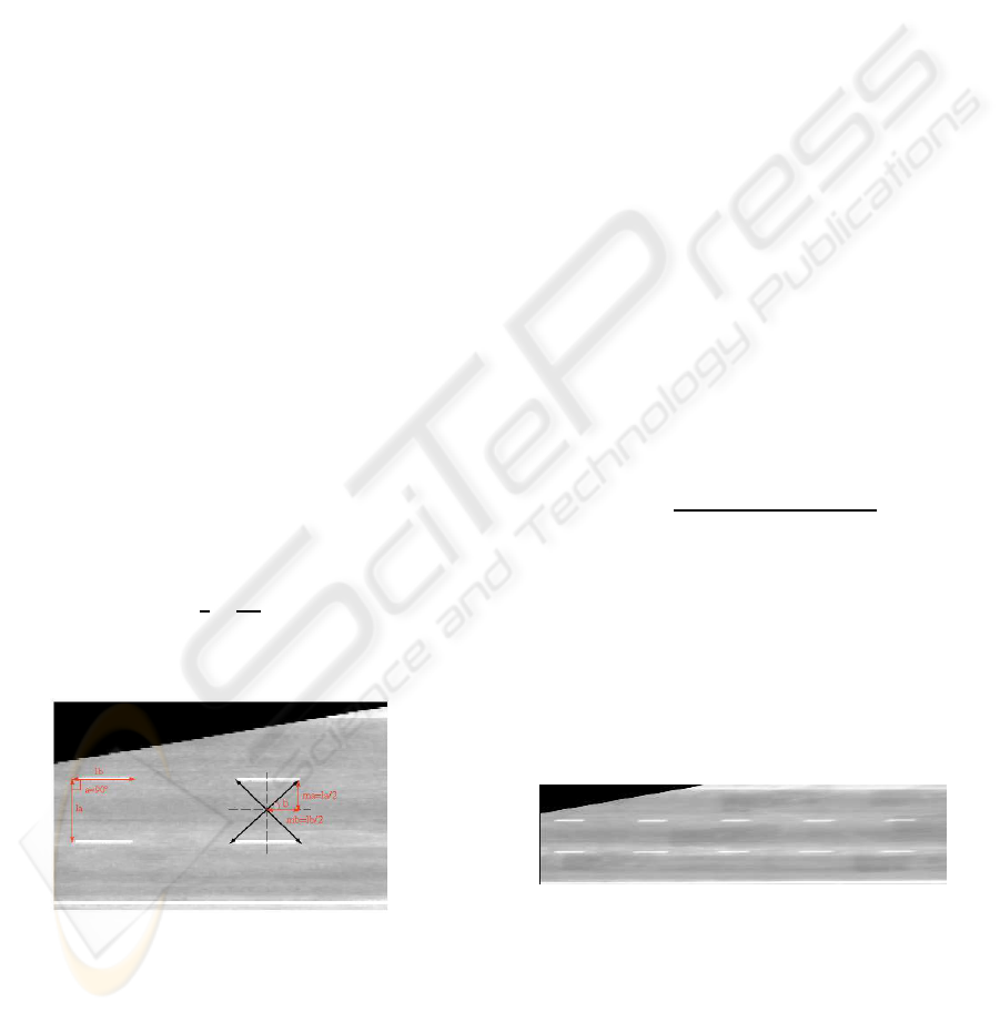
known angles. Figure 6 illustrates two possible angles

that can be used to calculate the required parameters

(α and β).





−α

0 1 0

0 0 1





(5)

Figure 6: Representation of two possible angles obtained

from two known lengths on the ground plane.

To conclude, the last transformation known as

similarity transformation performs rotation, transla-

tion and isotropic scaling of the resultant image.





s.cosθ −s.sinθ t

s.sinθ s.cosθ t

0 0 1





(6)

Therefore, a rectiﬁed image can be created by ap-

plying the following transformation, along with bilin-

ear interpolation, to each pixel of the image acquired

by the surveillance camera:

H = H

(7)

3 SCALE FACTOR AND LANE

PARAMETERS

Once the image sequence is rectiﬁed it is possible to

measure the distance, in kilometres, travelled by the

vehicle in two consecutive frames. In order to do so,

one must calculate a scale factor that relates pixels

in the image with the corresponding distance on the

ground plane. This scale factor can be obtained by es-

timating the ratio between the imaged highway stripe

period and the genuine stripe period on the ground

plane. Hence, in order to clearly identify the striped

lines on a rectiﬁed image plane, the previously at-

tained background image is rectiﬁed. Observing the

stripes presented on a rectiﬁed background image,

which can be seen on Figure 7, it is possible to con-

clude that these follow a periodic distribution. Us-

ing a auto correlation function, represented by expres-

sion (8), the lane stripe’s period can be located, since

the function has peaks in the beginning and ending of

each stripe, see Figure 8.

R(k) =

E [(X

− µ).(X

i+k

− µ)]

, (8)

where E is the expected value operator, X

is a

pixel of the straightened background image while

i+k

is a pixel on the same line of the referred image,

but distanced k pixels from the ﬁrst. µ represents the

average of the pixels of each line of the straightened

image, σ is the corresponding variance and k the al-

ready referred distance gap that, in this precise case,

is a number of columns of the rectiﬁed background

image.

Figure 7: Example of a straightened background image.

Therefore, the autocorrelation function is applied

to each line of the straightened background image, al-

lowing the identiﬁcation of the whereabouts and pe-

riods of the image stripes. Once located the image

highway stripes, it is possible to situate the highway

boundaries on the image plane. This information is

quite useful seeing as it may be used in estimating

each lane’s mean vehicle velocity.

VISAPP 2008 - International Conference on Computer Vision Theory and Applications

554

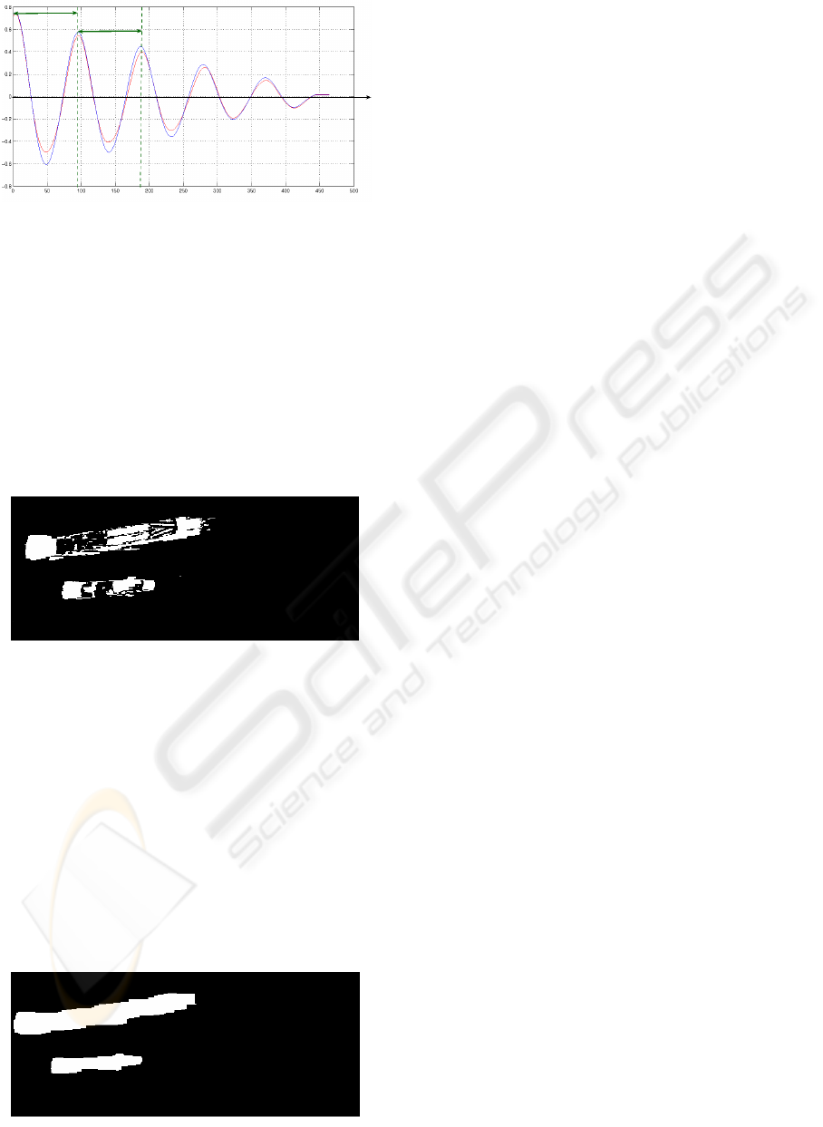
Figure 8: Autocorrelation functions of two stripe lines

present on the rectiﬁed background image The green arrows

represent the stripe period.

4 VEHICLE VELOCITY

To identify the location of vehicles on each frame, one

must ﬁrst distinguish objects from the background.

This procedure is known as image segmentation and

can be accomplished by subtracting each frame from

the background image. Figure 9 shows the result of

this operation.

Figure 9: Example of a segmented image.

However, as can be seen in Figure 9, this process

generates non-contiguous objects. This phenomenon

results from the lack of information in regions dis-

tant from the camera due to the perspective distortion

intrinsic in image formation. This fact is also respon-

sible for the visible deformation of vehicle shape on

rectiﬁed images. Seeing as non-contiguous objects

constitute a problem to vehicle detection, certain mor-

phological operations, such as dilation and erosion,

are applied to the resulting images. Figure 10 illus-

trates an example of a segmented image that may be

used in the identiﬁcation of vehicles.

Figure 10: Example of two continuous blobs.

The velocity associated with each detected ve-

hicle is easily attained by employing a Kalman ﬁl-

ter (Kalman and Bucy, 1960) based tracking sys-

tem. This process predicts future positions given a

sequence of images, and matches these with the in-

formation provided by blobs extracted from the seg-

mented image in order to correct the system’s model.

In order to do so, this process reiterates three steps

for each new frame. The ﬁrst step is responsible for

extracting the location of each identiﬁed vehicle us-

ing the contiguous object in the segmented image, ac-

knowledged as blob. Given two consecutive frames it

is possible to estimate motion, i.e. optical ﬂow, using

Lucas-Kanade’s method (Lucas and Kanade, 1981).

This technique presupposes that a pixel’s intensity is

invariant in two successive frames and therefore, it

is possible to determine motion by locating the cor-

responding pixel on the subsequent frame. Never-

theless, this method might be ﬂawed when applied

to trafﬁc image sequences. Consequently, we chose

to employ a Kalman ﬁlter to estimate each vehicle’s

position and correct the estimated velocity given by

Lucas-Kanade’s method. Given the fact that the im-

aged vehicles are travelling on a rectiﬁed image, their

velocity can be considered linear and therefore, the

following equations may be used to characterize a ve-

hicle’s movement:

i+1

= x

+ v

i+1

= y

+ v

.t (9)

where v

and v

represent the different velocity com-

ponents while x and y the vehicle’s position coordi-

nates. These expressions can be employed in the im-

plementation of the Kalman ﬁlter that estimates each

vehicle’s position and corrects the estimated velocity.

More precisely, each estimated state is obtained by

applying the following equation:

ˆx(k) = φ(k − 1).x(k− 1) =



x,v

,y,v



, (10)

where φ is the transition matrix and can be initially

deﬁned by the following matrix:

φ(0) =







1 1 0 0

0 1 0 0

0 0 1 1

0 0 0 1







(11)

This leads to the second step of the tracking sys-

tem. In order to employ a Kalman ﬁlter in this pro-

cess, one must relate a given estimation with the iden-

tiﬁed position using the segmented image. This pro-

cess is rather tricky due to the occasional overlapping

of blobs in the segmented image or absence of detec-

tion. Thus, a failsafe sub process was implemented in

order to deal with these cases.

ESTIMATING VEHICLE VELOCITY USING RECTIFIED IMAGES

555

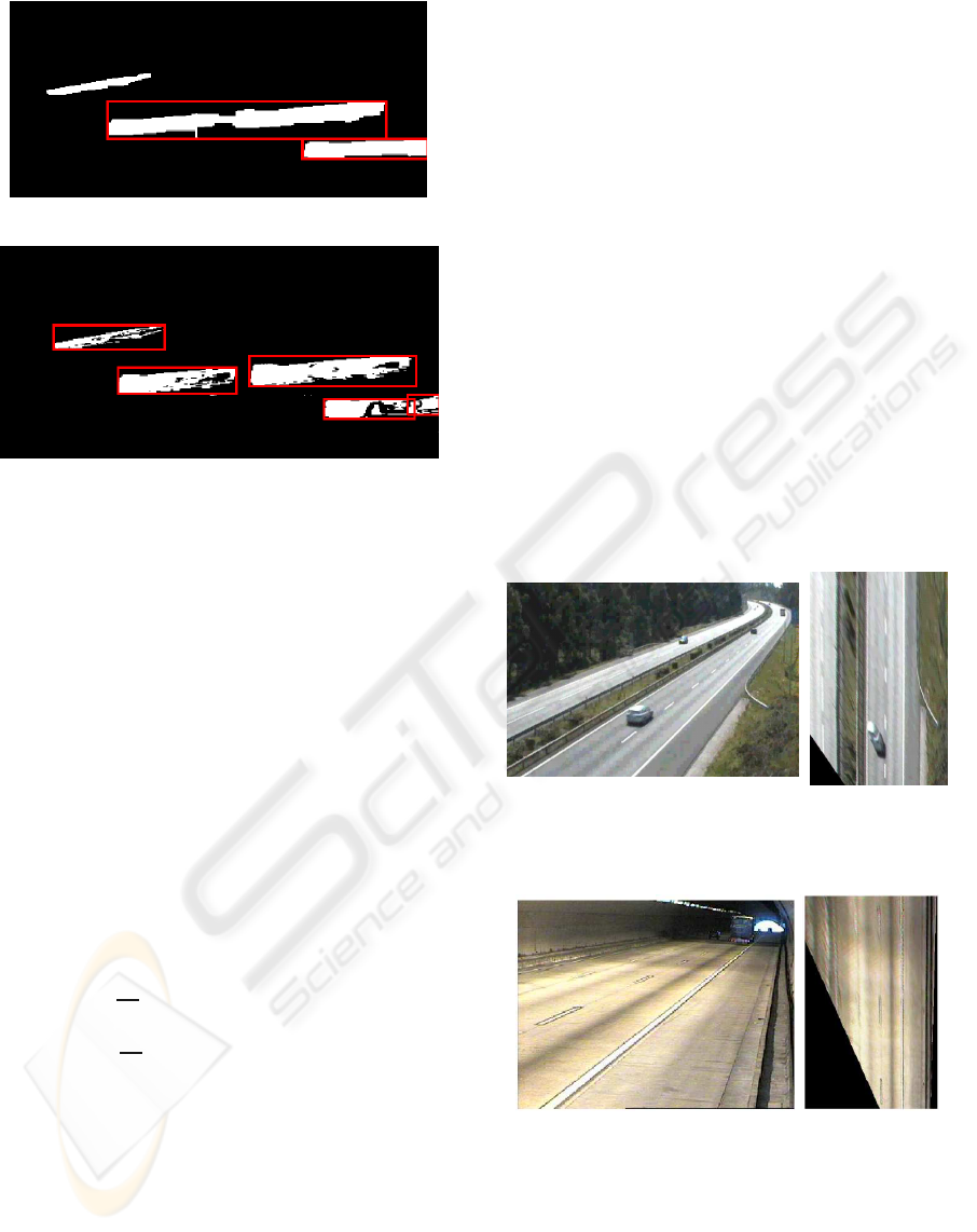
Figure 11: Representation of a blob overlying another.

Figure 12: Result of the employment of the failsafe process

to the image shown on Figure 11.

Figure 11 illustrates a segmented image where the

overlappingof two blobs is visible. On the other hand,

Figure 12 shows the result of the employment of fail-

safe process to image shown in Figure 11. As it can be

quite easily seen, the failsafe process does not employ

morphological operations to the segmented image and

uses more permissive parameters in the detection of

blobs. The ﬁnal step in this process uses the estimated

positions and estimated velocity provided from the

Kalman ﬁlter and performs data management. More

speciﬁcally, inserts new vehicles in to a linked list, re-

moves vehicles that are no longer acknowledged on

the segmented image or simply just updates data. In

this context, an object’s velocity is linear and there-

fore, once known the image sequence’s framerate, es-

timating vehicle velocity is quite straightforward, as

can be seen in the following expressions:

≃ 3, 6.∆x. f.s [km/h]

≃ 3,6.∆y. f.s [km/h] (12)

where ∆x and ∆y are the estimated displacements

in pixels between two consecutive images, s the

scale factor previously obtained and f the framerate.

Nonetheless, it is important to state that expression

(12) estimates vehicle velocity in kilometers per hour.

However, in order to obtain this estimation in another

unit system, the procedure is quite similar.

This application can also count the sum of vehicles

that travel on the observed scenario. To do so, an

analysis is made to a control ﬂag which indicates if

a vehicle hasn’t already been taken into account. The

referred analysis is preformed in the middle region of

the straightened image due to the fact that this region

has a higher probability of including all of the high-

way lanes. Given the fact that all the vehicles have

associated an identiﬁcation of the lane where these

pass through it is quite simple to calculate the mean

velocity of each lane.

5 RESULTS

In this section we present several rectiﬁed images and

two images that exemplify velocities obtained for sev-

eral vehicles on two consecutive images. Figures 13

and 14 illustrate the results of the employment of the

rectiﬁcation process to images captured by two differ-

ent surveillance cameras. The images on the left hand

side of each ﬁgure show the captured images to which

the process is applied, while the images on the right

hand side are the images achieved using the rectiﬁca-

tion process.

Figure 13: Example of a captured image (on the left) and

the correspondent rectiﬁed image (on the right).

Figure 14: Example of a captured image (on the left) and

the correspondent rectiﬁed image (on the right).

Figure 15 illustrates the tracking system in two

consecutive frames. In both images of this ﬁgure,

one may see each vehicles estimated velocity, the sum

of vehicles counted until that instant and each lanes

mean vehicle velocity which is represented on the up-

per left side of each image. Labeling each lane and

vehicle simpliﬁes the task of estimating each lanes

VISAPP 2008 - International Conference on Computer Vision Theory and Applications

556

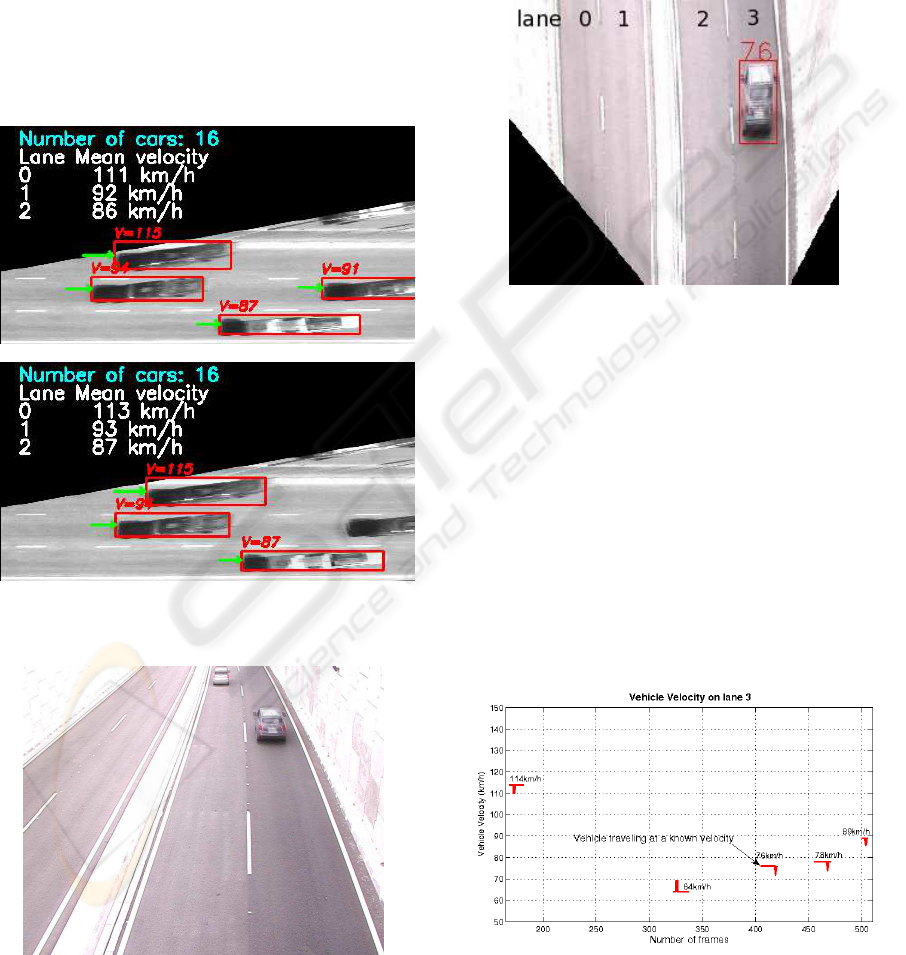
mean vehicle velocity. Therefore, each lane is identi-

ﬁed by an incremental numerical id. For instance, the

uppermost lane is labeled on the image as lane 0, the

lane below as lane 1 and ﬁnally the bottommost lane

as lane 2. By examining the mean vehicle velocity as-

sociated to each identiﬁed lane, one may observe that

the lane identiﬁed as lane 0 has the highest mean ve-

locity. Given the fact that this lane represents the ac-

celeration lane, this observation was not unexpected.

To conclude it is important to state that the green vec-

tors represented on each image of Figure 15 illustrate

the motion vectors for each identiﬁed vehicle, while

the estimated velocities in km/h are illustrated in red

above each vehicle.

Figure 15: Estimation of vehicle velocity in two consecutive

frames.

Figure 16: Captured image of the vehicle traveling at a

known velocity.

In order to establish the error associated to the ve-

hicle velocity estimation, the algorithm was applied

to a video sequence containing a vehicle traveling at

a known velocity. The referred vehicle is shown in

Figure 16 and was traveling at 74.5 km/h according

to a GPS system. To estimate this vehicle’s velocity

the rectiﬁcation process was applied as can be seen in

Figure 17. This Figure also shows the vehicle’s esti-

mated velocity between two consecutive frames.

Figure 17: Representation of the vehicle traveling at a

known velocity.

The result obtained applying the previously re-

ferred algorithm has an error of 2%, considering that

the vehicle’s real velocity was 74.5 km/h, measured

by a GPS system. The graphic represented in Figure

18 illustrates estimated velocities obtained by track-

ing several vehicles in consecutiveframes of the video

sequence represented in Figure 17. Analyzing this

Figure it is possible to observe that the instantaneous

velocities, estimated in each frame, are inﬂuenced by

noise caused by the lack of robustness of the segmen-

tation process. Figure 18 also represents the estimated

velocities of the vehicle traveling at a known velocity

on the ground plane.

Figure 18: Graphic illustrating the velocities of several ve-

hicles on lane 3.

ESTIMATING VEHICLE VELOCITY USING RECTIFIED IMAGES

557

6 CONCLUSIONS

This paper describes a technique to obtain a bird eye

view of the ground plane in order to estimate vehi-

cle velocity. The method requires no knowledge of

camera parameters, only needs two known lengths of

the highway. The rectiﬁcation technique also requires

that highway lanes and lane boundaries be approxi-

mately straight in the region of surveillance near the

camera. This method was tested on different trafﬁc

sequences, providing ﬁne results. To conclude, it is

important to state that this procedure can be employed

in other automatic trafﬁc surveillance systems.

REFERENCES

Bose, B. and Grimson, E. (2003). Ground plane rectiﬁ-

cation by tracking moving objects. In Proceedings

of the Joint IEEE International Workshop on Visual

Surveillance and Performance Evaluation of Tracking

and Surveillance.

Dailey, D. J. and Cathey, F. W. (2005). A novel technique to

dynamically measure vehicle speed using uncalibrated

roadway cameras. In Proceeding IEEE.

Fischler, M. A. and Bolles, R. C. (1981). Random sample

consensus: A paradigm for model ﬁtting with applica-

tions to image analysis and automated cartography. In

Comm.Assoc. Comp. Mach.

Kalman, R. E. and Bucy, R. S. (1960). New results in linear

ﬁltering and prediction theory. In Transactions of the

ASME, Journal of Basic Engineering (Series D).

Lazaros Grammatikopoulos, George Karras, E. P. (2002).

Automatic estimation of vehicle speed from uncali-

brated video sequences. In International Archives of

Photogrammetry and Remote Sensing.

Liebowitz, D. and Zisserman, A. (1998). Metric rectiﬁca-

tion for perspective images of planes. In Proceedings

of Computer Vision and Pattern Recognition.

Lucas, B. D. and Kanade, T. (1981). An iterative image

registration technique with an application to stereo vi-

sion. In Proceedings DARPA Image Understanding

Workshop.

Schoepﬂin, T. and Dailey, D. J. (2003). Dynamic camera

calibration of roadside trafﬁc management cameras

for vehicle speed estimation. In IEEE Transactions

on Intelligent Transportation Systems.

VISAPP 2008 - International Conference on Computer Vision Theory and Applications

558

REFERENCES

Bose, B. and Grimson, E. (2003). Ground plane rectifi-