MEAN SHIFT SEGMENTATION

Evaluation of Optimization Techniques

Jens N. Kaftan, Andr

e A. Bell and Til Aach

Institute of Imaging and Computer Vision, RWTH Aachen University, Templergraben 55, 52056 Aachen, Germany

Keywords:

Mean shift, segmentation, optimization, evaluation.

Abstract:

The mean shift algorithm is a powerful clustering technique, which is based on an iterative scheme to detect

modes in a probability density function. It has been utilized for image segmentation by seeking the modes in

a feature space composed of spatial and color information.

Although the modes of the feature space can be efﬁciently calculated in that scheme, different optimization

techniques have been investigated to further improve the calculation speed. Besides those techniques that

improve the efﬁciency using specialized data structures, there are other ones, which take advantage of some

heuristics, and therefore affect the accuracy of the algorithm output.

In this paper we discuss and evaluate different optimization strategies for mean shift based image segmen-

tation. These optimization techniques are quantitatively evaluated based on different real world images. We

compare segmentation results of heuristic-based, performance-optimized implementations with the segmen-

tation result of the original mean shift algorithm as a gold standard. Towards this end, we utilize different

partition distance measures, by identifying corresponding regions and analyzing the thus revealed differences.

1 INTRODUCTION

Image segmentation plays a crucial role in various

image processing applications in several domains, in-

cluding industrial as well as medical applications. It

describes the task of partitioning an image into sev-

eral segments or regions. Common segmentation ap-

proaches include simple thresholding techniques (Hu

et al., 2006), graph-based methods (Grady, 2006),

and level set techniques (Sethian, 1999) among oth-

ers. They have been applied to images from different

imaging modalities in typically two or three dimen-

sions, e.g., gray/color images, high dynamic range

images, CT/MR datasets, and multispectral images.

In general, these methods are adapted to the speciﬁc

application.

Mean shift is an unsupervised clustering algorithm

(Fukunaga and Hostetler, 1975), which estimates the

gradient of a probability density function to detect

modes in an iterative fashion. Hence, image segmen-

tations that take color/intensity-similarity as well as

local connectivity into account, can be obtained by

applying this algorithm to the combined spatial-range

domain (Comaniciu and Meer, 1997). Mean shift seg-

mentation has been successfully applied to several ap-

plications (Comaniciu and Meer, 1999; Suri et al.,

2002; Bell et al., 2006).

However, for larger images or applications where

processing time is very crucial, the mean shift seg-

mentation algorithm might be still too time consum-

ing. Based on the EDISON framework (Christoudias

et al., 2002; Comaniciu and Meer, 2002) we sum-

marize different optimization techniques for mean

shift based image segmentation. Given an applica-

tion for which the mean shift algorithm has proven

to be effective, one might now ask how these op-

timization techniques inﬂuence the segmentation re-

sults. Especially heuristic-based optimization tech-

niques alter the segmentation result and might affect

the applicability of the algorithm to the speciﬁc ap-

plication. Hence, we evaluate the segmentation re-

sults of performance-optimized compared to the non-

performance-optimized mean shift algorithm.

The paper is organized as follows. In Section 2 we

recapitulate the theoretical background of the mean

shift procedure. Subsequently, we present different

performance optimization techniques in Section 3. To

evaluate these heuristic-based performance optimiza-

tions with respect to the non-performance-optimized

mean shift segmentation we derive evaluation meth-

365

Kaftan J., Bell A. and Aach T. (2008).

MEAN SHIFT SEGMENTATION - Evaluation of Optimization Techniques.

In Proceedings of the Third International Conference on Computer Vision Theory and Applications, pages 365-374

DOI: 10.5220/0001085003650374

 SciTePress

ods in Section 4. Consequently, we apply these eval-

uation methods to several different image databases

and give numerical results in Section 5. Finally, we

conclude our results in Section 6.

2 THEORY

The mean shift algorithm (Fukunaga and Hostetler,

1975; Cheng, 1995) can be applied to a variety of

applications, including clustering, segmentation, and

ﬁltering (Comaniciu and Meer, 1997; Comaniciu and

Meer, 2002) and provides consistently good results

(Figure 1). The mean shift technique detects modes

in a probability density function based on the Parzen

Density Estimate (Fukunaga and Hostetler, 1975):

(x) =

∑

i=1



x − x



(1)

Here, N equals the number of d-dimensional vec-

tors x

..x

. The parameter h is the window radius

of the used kernel K

. In the domain of image seg-

mentation each feature vector is composed of the spa-

tial information of each pixel and the corresponding

color/intensity information in the range domain of di-

mension one or more.

The multivariate mean shift vector in the point x

is given by (Comaniciu and Meer, 2002)

(x) =

∑

i=1



x−x



∑

i=1



x−x



− x (2)

For the uniform kernel K

the calculation of the mean

shift vector (2) thus becomes an average of vector dif-

ferences. It can be shown that the mean shift vector

then is proportional to the normalized density gradi-

ent estimate (Comaniciu and Meer, 2002)

(x) =

∇

(x)

(3)

where c is the corresponding normalization constant

and K

is the radially symmetric Epanechnikov kernel

given by

(x) =

(

−1

(d + 2)(1 −

)

≤ 1

0 otherwise

(4)

with c

being a normalization constant.

To ensure the isotropy of the feature space, a uni-

form color space, such as the L

∗

is typically used.

In the case of grayvalue images, the L

∗

component is

used only. To account for different spatial and tonal

(a) Original (b) Mean shift segmented

Figure 1: Cameraman image. (a) Original. (b) Mean

shift segmented using high speedup level with (h

, h

) =

(32, 16).

variances it is reasonable to choose a kernel window

of size S

= S

with differing radii h

in the spatial

and h

in the range domain.

Since the mean shift vector is designed to be

aligned with the local gradient estimate, it can be

shown that by successive computation of (2) and shift-

ing the kernel window by m

(x), the mean shift pro-

cedure is guaranteed to converge to a point with zero

gradient, i.e., to a mode corresponding to the initial

position. Modes that are closer than h

and h

are

grouped together. For segmentation purposes, to each

pixel is then assigned the color/intensity value of the

corresponding mode. Furthermore, regions with less

than some pixelcount M might be optionally elimi-

nated.

The mean shift procedure is hence an effective

algorithm for mode seeking in a density distribution

without prior calculation of the distribution itself.

3 OPTIMIZATION TECHNIQUES

Although the mean shift vector can be calculated ef-

ﬁciently by just averaging the differences between

the current feature vector x and all feature vectors

within a certain space S

(x) around x, it is still ex-

pensive to identify the feature vectors falling into this

space for each mean shift vector calculation. This

problem is known as multidimensional range search-

ing (Georgescu et al., 2003).

Different performance optimizations have been

realized in the past. These mean shift variants reduce

computational time either by accelerating the calcula-

tion of one mean shift vector (category I) or by reduc-

ing the number of necessary mean shift vector cal-

culations (category II) or by combining both. Opti-

mizations that speed up the mean shift vector calcu-

lation often take advantage of specialized data struc-

tures and therefore do not affect the segmentation re-

VISAPP 2008 - International Conference on Computer Vision Theory and Applications

366

sult. Methods that reduce the number of necessary

mean shift vector calculations, however, usually use

heuristics, and therefore inﬂuence the quality of the

segmentation outcome.

For the Gaussian mean shift four different accel-

eration strategies have been examined in (Carreira-

Perpinan, 2006). The best speedup performance was

achieved by a spatial discretization step, which is very

similar to the mean shift vector reutilization technique

described in Section 3.2. With an optimal parameter

choice a speedup of factor 10x − 100x was achieved

with an error P < 3% (number of misclustered pixels

divided by the total number of pixels within the im-

age). Note that the Gaussian mean shift segmentation

is initially far slower to converge than the one using

the Epanechnikov kernel.

Based on the EDISON framework (Christoudias

et al., 2002; Comaniciu and Meer, 2002) that realizes

different mean shift optimizations using the Epanech-

nikov kernel, we detail these optimization techniques

in the following, which have also been shortly men-

tioned in (Christoudias et al., 2002).

While basic implementations of the mean shift

procedure usually work on the regular lattice struc-

ture of the image, one can improve the performance

utilizing an optimized ”bucket” structure that we de-

scribe in Section 3.1. This optimization of cate-

gory I signiﬁcantly increases the computational per-

formance without inﬂuencing the segmentation result.

Furthermore, we present two optimizations of cate-

gory II with medium (Section 3.2) and high (Sec-

tion 3.3) speedup level, respectively. Using all pos-

sible combinations - two realizations of category I

(lattice and bucket structure) × three of category II

(non-optimized (as described in Section 2), medium

speedup level, and high speedup level) - this sums up

to six different realizations.

3.1 Bucket Data Structure

One bottleneck of the mean shift procedure is the cost

per iteration, i.e., the cost of calculating the mean

shift vector for a given position x. The multidimen-

sional range searching problem, i.e., the identiﬁcation

of feature vectors within a certain space S

(x) around

x, is fairly straightforward on the regular lattice struc-

ture of an image within spatial range h

using a pro-

jection of S

(x) into the spatial domain S

(x) as a bi-

nary mask. Still, all those vectors need to be checked

if they are also within dynamic range h

, which is

computationally expensive even though the Epanech-

nikov kernel has a ﬁnite support.

This number of comparisons can be reduced with-

out impacting the result using a 3D bucket structure,

where each feature vector is assigned to the corre-

sponding 3D element of size h

× h

, a so called

”bucket” (in case the feature vector is of higher di-

mension than three, only the ﬁrst three elements are

used for data organization). Now, each feature vector

within S

(x) is guaranteed to be within the same or

a neighboring bucket of x. This discretization of the

feature vectors into buckets allows for easy identiﬁ-

cation of feature vectors that are farther than 2 · h

2 · h

away from x, and thus do not need to be consid-

ered any further. Hence, the number of comparisons

is reduced on average.

3.2 Mean Shift Vector Reutilization

Another bottleneck of the mean shift procedure is the

number of iterations to identify the mode correspond-

ing to the initial position x. Using the non-optimized

mean shift deﬁnition, the mean shift vector is calcu-

lated and added to the current feature vector until con-

vergence. This is repeated for each point within the

image. Thus if we start the mean shift process from

a data point x

, at some iteration τ the current feature

vector x

(τ)

might become equal (or very similar) to

another feature vector x

and hence both x

and x

share the same fate, i.e., converge to the same mode.

Such information is not exploited in the basic version,

so that the mean shift vector of certain positions might

be calculated several times, especially for positions

close to a mode, that are typically traversed by many

paths (iteration steps starting from a position x).

Using this optimization, the closest point (i.e.,

the spatially nearest neighbor) to the current feature

vector x

(τ)

at each iteration step τ, which we refer

to as x

candidate

in the following, is considered and if

candidate

is within a distance of ε

· h

to the current

feature vector x

(τ)

, both points are assigned to the

same mode. Because of the regular grid of the im-

age and the uniform kernel chosen to calculate the

mean shift vector, it is obvious that a feature vector

(τ)

converges to the same mode as its nearest neigh-

bor x

candidate

on the grid if both feature vectors are

identical in their range domain (after quantization of

the range part of x

(τ)

into the image range domain).

If both vectors are not equal but very similar in their

range domain, however, this is not always true, but

a reasonable assumption. Now, in case the corre-

sponding mode to x

candidate

has already been calcu-

lated, the iteration can be stopped early, while other-

wise x

candidate

can be assigned to the same mode as

the initial feature vector x

Compared to this optimization technique, the spa-

tial discretization step (Carreira-Perpinan, 2006) sub-

MEAN SHIFT SEGMENTATION - Evaluation of Optimization Techniques

367

divides each pixel into l × l cells. Each data point

that projects onto a cell at some iteration τ

does

converge to the same mode as any other point x

that

projects onto the same cell at some iteration τ

, inde-

pendent of the range domain.

This mean shift vector reutilization technique is

called ”medium speedup” in the EDISON framework.

The parameter ε

can be freely chosen and is preset to

= 0.5. A low factor will result in a small speedup

and a high segmentation accuracy compared to the

non-optimized case and vice versa.

3.3 Local Neighborhood Inclusion

Additionally to the heuristic described in Section 3.2

one can extend the idea of forcing feature vectors x

(τ)

and x

candidate

that are identical in their spatial domain

(after quantization into the image grid) and similar

in their range domain to converge to the same mode

into forcing feature vectors that are similar in both

domains. That means that additionally all feature

vectors within S

(τ)

) are checked if their distances

are smaller than ε

· h

to x

(τ)

. Then, in analogy to

the above described method, feature vectors x

candidate

within ε

· h

distance that are not yet assigned to an-

other mode get assigned to the same mode as the cur-

rent feature vector x

(τ)

. In case one vector candidate

has already been assigned to a mode, the iteration pro-

cess for x

can be again stopped early.

As this optimization strategy, called ”high

speedup” in the EDISON framework, is more error-

prone than the mean shift vector reutilization it is rea-

sonable to choose the parameter ε

< ε

(ε

is preset

to 0.1).

4 EVALUATION METHOD

Assuming the mean shift segmentation results are

satisfying for a given application, we are interested

in how much the heuristics of the performance-

optimized mean shift segmentation will alter the seg-

mentation result. The performance optimizations

covered in Section 3.2 and 3.3 will in this respect

introduce ”errors” compared to the non-optimized

mean shift segmentation result. Hence, to exam-

ine the inﬂuence of these optimization techniques on

the mean shift segmentation, we use the original,

non-optimized mean shift segmentation as reference,

which we will call the ”original” result in the follow-

ing. To simplify matters, we limit the evaluation to

single channel 2D images, but one can easily trans-

fer the following methods and results to multichannel

and multidimensional images.

As the mean shift algorithm partitions the image

into several segments rather than separating an ob-

ject (foreground) from the background, typical evalu-

ation features based on the well-known true/false pos-

itive/negative notation (Udupa et al., 2002) cannot be

used for validation purposes. It is also not sufﬁcient

to analyze the difference of both resulting images to

compare different mean shift methods in the domain

of image segmentation. In this particular case the ob-

ject boundaries of all resulting regions are relevant.

To identify erroneous segmented areas one needs to

ﬁnd corresponding regions in both resulting images,

i.e., the original and comparison segmentation (see

Section 4.1). Then, those pixels at identical image

position that belong to non corresponding regions are

erroneous segmented and can be further analyzed (see

Section 4.2).

4.1 Corresponding Regions

In the output images of the segmentation step, each

region is colored by the gray value of the correspond-

ing mode. As multiple modes may have the same gray

value we ﬁrstly label each connected region of pixels

of identical gray value with an unique ID resulting in

two partitions: O for the original and C for the com-

parison result. To identify corresponding regions, the

number of pixels at identical image positions that be-

long to region c

∈ C, i ∈ [0, n − 1] and o

∈ O, o ∈

[0, m − 1] are counted with n, m being the total num-

ber of regions in C and O, respectively. These pixel-

counts are then stored within a joint-histogram or cor-

respondence matrix A(O,C) := (a

i, j

)

n×m

as elements

at position (i, j). In the following refers one row i to

the pixelcounts of one region c

in C and one column

j to the pixelcounts of one region o

in O. The iden-

tiﬁcation of corresponding regions equals an optimal

assignment problem that can be deﬁned in different

manners (Cardoso and Corte-Real, 2005):

Each region in C corresponds to a maximum of

one region in O and vice versa. Then, O and C are

identical if and only if each corresponding pair of re-

gions is identical and when there are no regions with-

out correspondence left. Otherwise, the partition dis-

tance d

sym

(O,C) equals the sum of pixels that belong

to non corresponding regions in O and C and pixels of

regions without correspondence. In other words, the

symmetric partition distance equals

sym

(O,C) = t − v(O,C) (5)

with t being the total number of pixels and v(O,C)

denoting the value of the assignment (Cardoso and

Corte-Real, 2005), which is the sum of a selection of

VISAPP 2008 - International Conference on Computer Vision Theory and Applications

368

(a) Partition O (b) Partition C

Figure 2: The right partition is a reﬁnement of the left par-

tition.

elements a

i, j

of A(O,C) such that no row or column

contains more than one selected element. The optimal

assignment is that one of all possible ones that mini-

mizes the symmetric partition distance d

sym

(O,C) and

consequently maximizes the number of pixels v(O,C)

at identical image positions that belong to correspond-

ing regions c

, o

. This assignment problem is solved

based on the Hungarian method (Kuhn, 1955) and re-

sults in a one-to-one matching.

Alternatively the maximum element in each row

max

A(O,C) ∀ i can be located and used to assign

corresponding regions c

, o

. Such strategy, however,

can result in a many-to-one matching (Kaftan et al.,

2006). In other words, if a region o

within the origi-

nal partition falls apart into two or more different re-

gions, many regions c

within the comparison parti-

tion might be assigned to o

, allowing an oversegmen-

tation of C compared to O. Then, C is a reﬁnement

(Cardoso and Corte-Real, 2005) of O (or C is ﬁner

than O) if and only if each region c

in C is identical

to or is contained in one region o

in O (see Figure 2).

The resulting asymmetric partition distance

asy

(O,C) can be obtained straightforward from ma-

trix A(O,C) as

asy

(O,C) = t −

∑



max

A(O,C)



(6)

Under this asymmetric distance, any partition ﬁner

than the partition O will be at zero distance from it.

Notice that, in general, d

asy

(O,C) 6= d

asy

(C, O).

The other asymmetric distance d

asy

(C, O) can be

calculated accordingly by locating the maximum ele-

ment in each column of A(O,C)

asy

(C, O) = t −

∑



max

A(O,C)



(7)

Under this asymmetric distance, any partition C for

which O is an reﬁnement will be at zero distance from

it and hence allows an undersegmentation of C com-

pared to O.

The optimal strategy, however, depends on the

intended application, because different error types

might have unequal strong effects on the overall per-

formance.

4.2 Evaluation Features

Once corresponding regions have been identiﬁed, the

revealed differences can be analyzed. For qualitative

evaluation we show binary error images wherein each

missegmented pixel is colored in black. For quantita-

tive evaluation we have furthermore calculated differ-

ent features:

For segmentation purposes it is important how the

errors are distributed over the image. If many isolated

pixels are evenly spread it might not be as severe as

large connected regions being missegmented. Hence,

we applied a connected component analysis to the re-

sulting error images and calculated the average region

size A

region

and its standard deviation.

Using the mean shift procedure as edge preserv-

ing ﬁltering technique, however, does not necessarily

need a large overlap of corresponding regions. For

such an application the grayvalue differences might

be more meaningful and hence we calculate the mean

grayvalue difference of missegmented pixels between

the original and comparison ﬁlter output.

5 RESULTS

We have evaluated optimization techniques based on

several real world images from different databases

(see Figure 3). In the domain of object segmenta-

tion we have used the publicly available databases

COIL-20 and COIL-100 (Nene et al., 1996a; Nene

Figure 3: Example images from the COIL, CELL, and

MISC databases, respectively.

MEAN SHIFT SEGMENTATION - Evaluation of Optimization Techniques

369

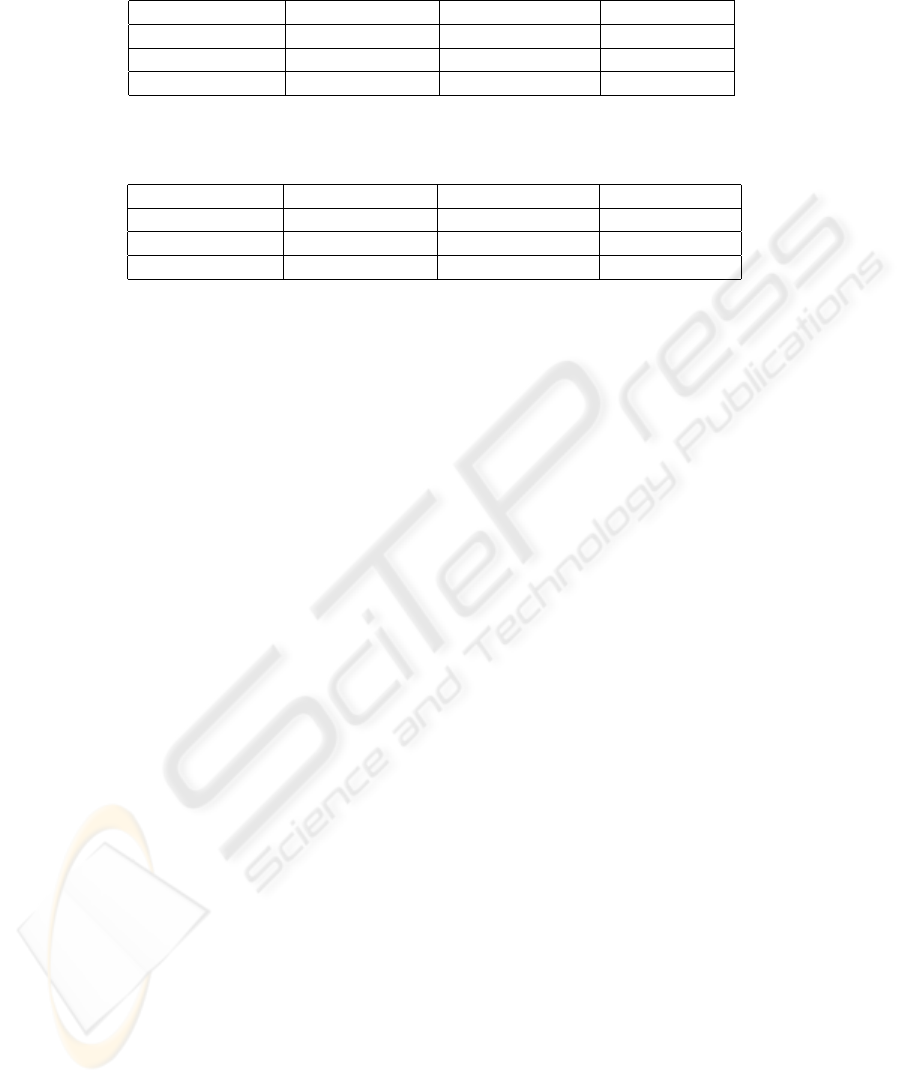
Table 1: Processing times for the Cameraman image (256x256 Pixel, 256 grayvalues, Figure 1) using the lattice data structure

(ε

= 0.5, ε

= 0.1) as absolute time (in seconds) and relative to the non-optimized version using the lattice structure.

Parameters No optimization Medium speedup High speedup

= 8, h

= 4 6.575 (1.0) 1.704 (0.26) 0.239 (0.04)

= 16, h

= 8 40.574 (1.0) 5.997 (0.15) 0.333 (0.008)

= 32, h

= 16 279.530 (1.0) 17.343 (0.06) 0.281 (0.001)

Table 2: Processing times using the bucket data structure (ε

= 0.5, ε

= 0.1) as absolute time (in seconds) and relative to the

non-optimized version using the lattice structure as listed in Table 1.

Parameters No optimization Medium speedup High speedup

= 8, h

= 4 5.471 (0.83) 0.933 (0.14) 0.214 (0.03)

= 16, h

= 8 27.075 (0.67) 2.949 (0.07) 0.229 (0.006)

= 32, h

= 16 180.909 (0.64) 8.471 (0.03) 0.219 (0.0008)

et al., 1996b). Each available object was segmented

at grayscale level using three different rotations, sum-

marizing to a total of 360 images (in the following

referred to as COIL-database). In the medical domain

we have examined 200 brightﬁeld light microscopy

cell images (Bell et al., 2006) from human oral mu-

cosae in Feulgen and Silver staining each (CELL-

database). Additionally we have used a set of 20 dif-

ferent images, cropped and scaled to a common im-

age size to allow a better comparison, that have been

used in earlier publications (see especially (Comani-

ciu and Meer, 1999)) to show the effectiveness of the

original mean shift procedure (MISC-database). Each

performance-optimized segmentation has been vali-

dated (see Section 5.1 and Section 5.2) in comparison

to the original result as reference. Since the used data

structure does not inﬂuence the segmentation result,

we have used the bucket structure (see Section 3.1)

for all experiments analyzing the segmentation accu-

racy. The computational efﬁciency has been exam-

ined using all possible permutations of optimization

techniques. Considering both aspects, segmentation

quality and computation time, allows to rate the ap-

plicability of each technique to the application of in-

terest, based on its requirements.

To measure the processing time, the Cameraman

image (256x256 Pixel, 256 grayvalues, Figure 1) has

been processed using various spatial and range kernel

radii on a Pentium 4, 3.4GHz. The results averaged

over three runs are shown in Table 1 using the lattice

and in Table 2 using the bucket structure. Addition-

ally to the absolute times (in seconds) the relative time

according to the non-optimized version using the lat-

tice structure are listed.

5.1 Segmentation Quality

To evaluate the segmentation quality, each image

has been segmented without using optional post-

processing steps to avoid their inﬂuence on the seg-

mentation output. Using the mean shift procedure

alone, however, will still result in an image contain-

ing several very small regions depending on the ker-

nel size. To circumvent the image falling apart into

too many regions we have chosen relatively large ker-

nel sizes (h

, h

) = (15, 25). The parameters of the

optimization techniques have been set to ε

= 0.5 and

= 0.1.

To quantify the differences between the non-

optimized and optimized versions of the mean shift

procedure, the resulting images have been compared

using the symmetric partition distance d

sym

(O,C)

and both asymetric partition distances d

asy

(O,C) and

asy

(C, O), which allow the optimized result to be

oversegmented, resp. undersegmented compared to

the original result. The resulting difference images

are exemplarily shown in Figure 4. Averaged over all

test images the relative number on missegmented pix-

els ranges between 4.6% and 18.2% for the mean shift

vector reutilization and between 6.2% and 23.6% for

the local neighborhood inclusion technique depend-

ing on the chosen partition distance and database (see

Table 3).

However, as the test set includes different images,

it is difﬁcult to compare the absolute number of mis-

segmented pixels for both optimization techniques.

Looking at each individual image, we have therefore

calculated the relative increase of missegmented pix-

els of the local neighborhood inclusion technique in

relation to the number of missegmented pixels us-

ing the mean shift vector reutilization technique and

hence obtain a measure that considers the complex-

ity of the segmentation task. Determining the median

VISAPP 2008 - International Conference on Computer Vision Theory and Applications

370

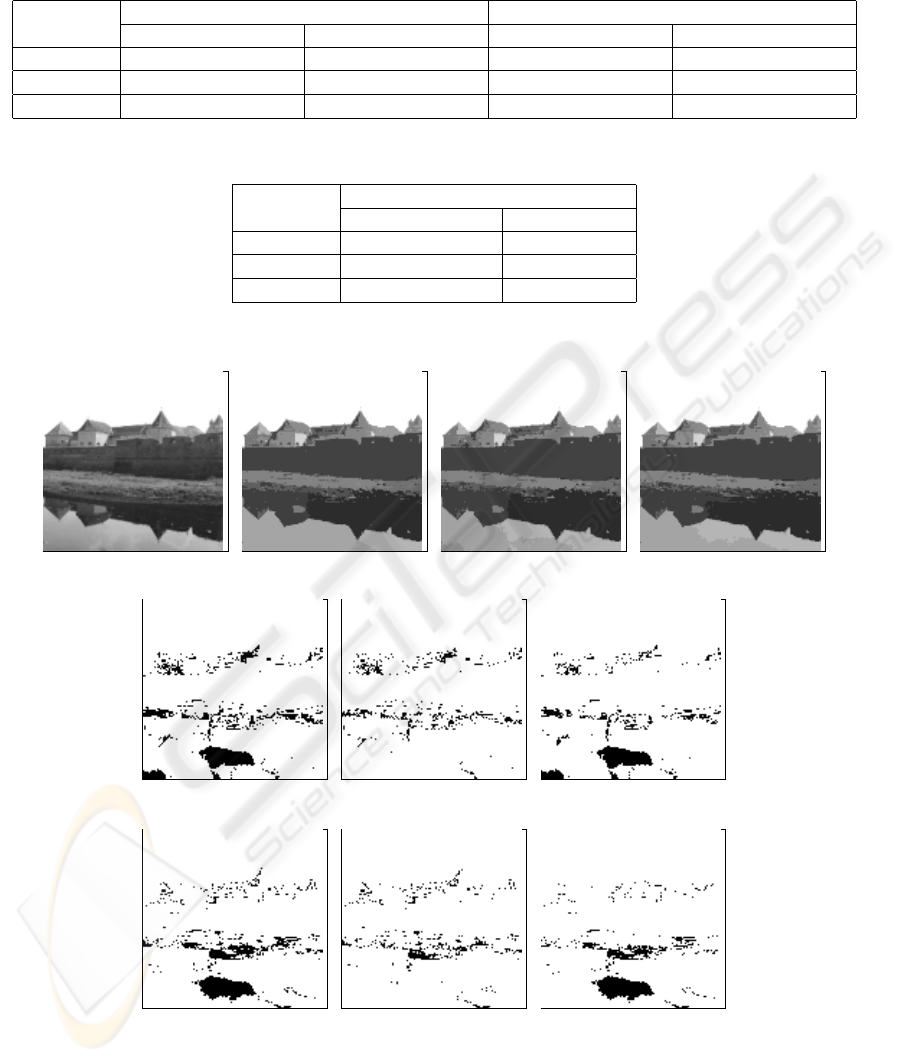
Table 3: Averaged segmentation error. For each optimization technique, the partition distances are listed as absolute pixel

count and relative to the image size (mean value ± standard deviation). Note that the image size within one database is

constant while varying between different databases.

MISC-database COIL-database

Medium speedup High speedup Medium speedup High speedup

sym

(O,C) 2807 (18.0±11.2%) 3163 (20.2±10.2%) 2217 (13.5±11.7%) 2802 (17.1±12.7%)

asy

(O,C) 1209 (7.7±4.2%) 1433 (9.2±5.2%) 841 (5.1±5.5%) 1167 (7.1±7.1%)

asy

(C, O) 2120 (13.6±10.8%) 2333 (14.9±8.3%) 1738 (10.6±10.6%) 2124 (13.0±11.0%)

Averaged segmentation error relative to the image size (image size varies within CELL-database).

CELL-database

Medium speedup High speedup

sym

(O,C) 18.2±14.2% 23.6±15.1%

asy

(O,C) 4.6±4.0% 6.2±5.6%

asy

(C, O) 15.8±13.5% 20.3±14.1%

(a) Original (b) Non-optimized (c) Medium speedup (d) High speedup

(e) d

sym

(O,C) (f) d

asy

(O,C) (g) d

asy

(C, O)

(h) d

sym

(O,C) (i) d

asy

(O,C) (j) d

asy

(C, O)

Figure 4: (a) Fagaras image. (b-d) Mean shift segmented using different speedup levels with (h

, h

) = (15, 25). (e-g) Partition

distance of (c) and (b). (h-j) Partition distance of (d) and (b) (missegmented pixels are shown in black color).

MEAN SHIFT SEGMENTATION - Evaluation of Optimization Techniques

371

Table 4: Averaged size of missegmented regions in pixel. The common image sizes of the MISC- and COIL-database are

125x125, and 128x128 respectively. The averaged standard deviation of the region sizes within each image is listed in

brackets.

MISC-database COIL-database

Medium speedup High speedup Medium speedup High speedup

sym

(O,C) 19.2 (137.3) 17.7 (143.7) 67.6 (233.7) 66.0 (299.3)

asy

(O,C) 6.1 (26.0) 6.8 (37.4) 14.5 (48.9) 12.2 (69.0)

asy

(C, O) 16.6 (119.3) 14.4 (117.2) 83.3 (209.1) 66.9 (252.9)

Averaged size of missegmented regions relative to the image size on the CELL database. The averaged standard deviation of

the relative region sizes within each image is listed in brackets.

CELL-database

Medium speedup High speedup

sym

(O,C) 0.26 (3.3) 0.33 (4.0)

asy

(O,C) 0.04 (0.2) 0.06 (0.4)

asy

(C, O) 0.32 (4.9) 0.35 (4.9)

Table 5: Averaged mean difference between the grayvalues of missegmented pixels compared to the non-optimized segmen-

tation result in absolute values and relative to the dynamic range (mean value ± standard deviation).

MISC-database COIL-database

Medium speedup High speedup Medium speedup High speedup

sym

(O,C) 14.5 (5.7±2.0%) 14.0 (5.5±2.1%) 19.5 (7.6±2.9%) 19.7 (7.7±3.0%)

asy

(O,C) 17.4 (6.8±2.4%) 16.5 (6.5±2.4%) 22.6 (8.8±3.0%) 22.0 (8.6±3.6%)

asy

(C, O) 14.9 (5.8±2.1%) 14.7 (5.7±2.5%) 20.5 (8.0±3.2%) 21.6 (8.4±3.3%)

Averaged mean grayvalues difference on the CELL database.

CELL-database

Medium speedup High speedup

sym

(O,C) 15.3 (6.0±2.3%) 14.3 (5.6±2.0%)

asy

(O,C) 21.0 (8.2±2.0%) 19.9 (7.8±2.3%)

asy

(C, O) 16.2 (6.3±3.3%) 14.8 (5.8±3.0%)

value of this measure shows that the number of mis-

segmented pixels grows by 24.7% using the symmet-

ric distance measure and by 19.7% and 24.3% using

asy

(O,C) and d

asy

(C, O), respectively.

Next, the average missegmented region size did

not signiﬁcantly change between the optimization

techniques. However the increased averaged standard

deviation of the region sizes within each image indi-

cates that the local neighborhood inclusion techniques

produces a larger variance (d

sym

(O,C) and d

asy

(O,C))

and hence also larger connected regions of misseg-

mented pixel than the mean shift vector reutilization

technique (see Table 4).

Finally, the average mean difference of the mis-

segmented pixel gray values compared to the non-

optimized segmentation result did not change signiﬁ-

cantly (see Table 5).

5.2 Rotational Invariance

The heuristic-based optimization techniques both ac-

cess earlier calculated mean shift vectors to estimate

the correct mean shift vector at some positions and

hence result in a mean shift procedure, which is not

rotationally invariant anymore. In fact, the order-

ing of the pixels being processed may have a sig-

niﬁcant impact on the segmentation result. To ver-

ify this observation, we have exemplarily rotated one

image by 90

◦

and compared its segmentation using

, h

) = (15, 25) for each optimization technique to

the segmentation result of the non-rotated image. Fig-

ure 5 shows on the basis of the error images using the

symmetric partition distance that the local neighbor-

hood inclusion technique is stronger corrupted (as ex-

pected) than the mean shift vector reutilization tech-

nique, while the non-optimized version can be con-

VISAPP 2008 - International Conference on Computer Vision Theory and Applications

372

(a) Original (b) Non-optimized (c) Medium speedup (d) High speedup

(e) Rotated, non-optimized (f) Rotated, med. speedup (g) Rotated, high speedup

(h) d

sym

(O,C) (i) d

sym

(O,C) (j) d

sym

(O,C)

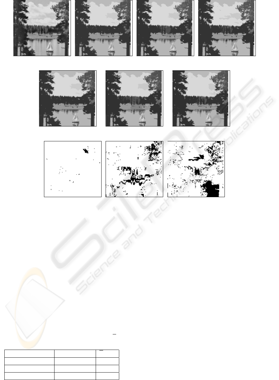
Figure 5: (a) Lake image. (b-d) Mean shift segmented using different speedup levels with (h

, h

) = (15, 25). (d-f) Mean

shift segmented using identical parameters, but a 90

◦

rotated input image. (h-j) Partition distance of (b-d) and (e-g) using

sym

(O,C) comparing corresponding optimization techniques.

sidered to be practically rotationally invariant. In fact,

even for the non-optimized version, a few error pixels

can be observed due to numerical reasons. Analyzing

the error images shows (see Table 6) that 16.1% of the

pixels are affected using the local neighborhood in-

clusion speedup technique and 11.1% using the mean

shift vector reutilization technique (compared to 0.6%

for the non-optimized version) with an average region

size of 10.56 and 9.75 pixels, respectively.

Table 6: Segmentation error caused by rotational variance.

For each optimization technique, the symmetric partition

distance d

sym

(O,C) and the average error region size A

region

are listed from the images shown in Figure 5.

Optimization d

sym

(O,C) A

region

Non-optimized 96 (0.6%) 3.84

Medium speedup 1742 (11.1%) 10.56

High speedup 2516 (16.1%) 9.75

6 CONCLUSIONS

We have quantitatively evaluated different optimiza-

tion techniques for the Epanechnikov based mean

shift segmentation algorithm regarding their accuracy

and computational performance. As expected, each

optimization technique that reduces the number of

necessary mean shift vector calculations introduces

some errors compared to the non-optimized mean

shift procedure. On the one hand, the quantity of er-

rors has been measured to be on average 18.0% for the

mean shift vector reutilization and 20.2% for the local

neighborhood inclusion technique using a symmetric

partition distance measure. However, the impact of

such optimizations on the segmentation accuracy de-

pends on the image material. Depending on the ap-

plication the fact that using the described heuristics

results in a rotationally variant segmentation (up to

16.1% of the pixels have been affected in our exam-

ple) might be even more severe than the previously

MEAN SHIFT SEGMENTATION - Evaluation of Optimization Techniques

373

mentioned errors. On the other hand, the improve-

ment of the computational efﬁciency is remarkable.

Especially for large kernel radii, the processing time

could be reduced from 280s to 0.219s on a standard

PC in our example. Finally, it depends on the require-

ments of the intended application if the described op-

timization techniques are applicable but analyzing our

results one can rate the pros and cons of each tech-

nique.

ACKNOWLEDGEMENTS

We would like to thank the authors of

(Christoudias et al., 2002) for providing the

EDISON software at their laboratory website

(http://www.caip.rutgers.edu/riul/) and the authors of

(Cardoso and Corte-Real, 2005) for providing their

evaluation application upon request.

REFERENCES

Bell, A. A., Kaftan, J. N., Aach, T., Meyer-Ebrecht, D., and

ocking, A. (2006). High Dynamic Range Images as

a Basis for Detection of Argyrophilic Nucleolar Or-

ganizer Regions Under Varying Stain Intensities. In

IEEE International Conference on Image Processing.

ICIP 2006, pages 2541–2544.

Cardoso, J. and Corte-Real, L. (2005). Toward a generic

evaluation of image segmentation. IEEE Transactions

on Image Processing, 14(11):1773–1782.

Carreira-Perpinan, M. A. (2006). Acceleration strategies for

gaussian mean-shift image segmentation. In Proceed-

ings of the 2006 IEEE Computer Society Conference

on Computer Vision and Pattern Recognition. CVPR

2006, pages 1160–1167.

Cheng, Y. (1995). Mean Shift, Mode Seeking, and Clus-

tering. IEEE Transactions on Pattern Analysis and

Machine Intelligence, 17(8):790–799.

Christoudias, C. M., Georgescu, B., and Meer, P. (2002).

Synergism in Low Level Vision. In IEEE Inter-

national Conference on Pattern Recognition. ICPR

2002, volume 4, pages 150–155.

Comaniciu, D. and Meer, P. (1997). Robust Analysis of

Feature Spaces: Color Image Segmentation. In IEEE

Conference on Computer Vision and Pattern Recogni-

tion. CVPR 1997, pages 750–755.

Comaniciu, D. and Meer, P. (1999). Mean Shift Analysis

an Applications. In International Conference on Com-

puter Vision. ICCV 1999, volume 2, pages 1197–1203.

Comaniciu, D. and Meer, P. (2002). Mean Shift: A Ro-

bust Approach Toward Feature Space Analysis. IEEE

Transactions on Pattern Analysis and Machine Intel-

ligence, 24(5):603–619.

Fukunaga, K. and Hostetler, L. D. (1975). The Estimation

of the Gradient of a Density Function, with Applica-

tions in Pattern Recognition. IEEE Transactions on

Information Theory, 21(1):32–40.

Georgescu, B., Shimshoni, I., and Meer, P. (2003). Mean

Shift Based Clustering in High Dimensions: A Tex-

ture Classiﬁcation Example. In International Con-

ference on Computer Vision. ICCV 2003, volume 1,

pages 456–463.

Grady, L. (2006). Random walks for image segmentation.

IEEE Transactions on Pattern Analysis and Machine

Intelligence, 28(11):1768–1783.

Hu, Q., Hou, Z., and Nowinski, W. L. (2006). Supervised

range-constrained thresholding. IEEE Transactions

on Image Processing, 15(1):228–240.

Kaftan, J. N., Kiraly, A. P., Naidich, D. P., and Novak, C. L.

(2006). A Novel Multi-Purpose Tree and Path Match-

ing Algorithm with Application to Airway Trees. In

SPIE Medical Imaging 2006: Physiology, Function,

and Structure from Medical Images, volume 6143,

pages 215–224.

Kuhn, H. W. (1955). The Hungarian method for the assign-

ment problem. Naval Research Logistic Quarterly,

2:83–97.

Nene, S., Nayar, S., and Murase, H. (1996a). Columbia

Object Image Library (COIL-100). Technical report,

Computer Vision Laboratory, Columbia University.

Nene, S., Nayar, S., and Murase, H. (1996b). Columbia Ob-

ject Library (COIL-20). Technical report, Computer

Vision Laboratory, Columbia University.

Sethian, J. A. (1999). Level Set Methods and Fast Marching

Methods. Cambridge University Press.

Suri, J. S., Setarehdan, S. K., and Singh (Eds), S. (2002).

Advanced Algorithmic Approaches to Medical Image

Segmentation. Springer.

Udupa, J. K., LaBlanc, V. R., Schmidt, H., Imielinska, C.,

Saha, P. K., Grevera, G. J., Zhuge, Y., Currie, L. M.,

Molholt, P., and Jin, Y. (2002). Methodology for eval-

uating image-segmentation algorithms. In SPIE Med-

ical Imaging: Image Processing, volume 4684, pages

266–277.

VISAPP 2008 - International Conference on Computer Vision Theory and Applications

374