OMNIDIRECTIONAL CAMERA MOTION ESTIMATION

Akihiko Torii and Tom´aˇs Pajdla

Center for Machine Perception, Department of Cybernetics, Faculty of Elec. Eng.

Czech Technical University in Prague, Karlovo n´am. 13, 121 35, Prague, Czech Republic

Keywords:

Camera Motion Estimation, Omnidirectional Images, Epipolar Geometry.

Abstract:

We present an automatic technique for computing relative camera motion and simultaneous omnidirectional

image matching. Our technique works for small as well as large motions, tolerates multiple moving objects

and very large occlusions in the scene. We combine three principles and obtain a practical algorithm which

improves the state of the art. First, we show that the correct motion is found much sooner if the tentative

matches are sampled after ordering them by the similarity of their descriptors. Secondly, we show that the

correct camera motion can be better found by soft voting for the direction of the motion than by selecting

the motion that is supported by the largest set of matches. Finally, we show that it is useful to ﬁlter out the

epipolar geometries which are not generated by points reconstructed in front of cameras. We demonstrate the

performance of the technique in an experiment with 189 image pairs acquired in a city and in a park. All

camera motions were recovered with the error of the motion direction smaller than 8

◦

, which is 4 % of the

183

◦

ﬁeld of view, w.r.t. the ground truth.

1 INTRODUCTION

Projections of scene points into images acquired by

a moving camera are related by epipolar geome-

try (Hartley and Zisserman, 2004). In this work, we

present a practical algorithm which improves the state

of the art automatic camera relative motion computa-

tion and simultaneous image matching. Such an algo-

rithm is a useful building block for autonomous nav-

igation and building large 3D models using structure

from motion.

In contrary to existing structure from motion al-

gorithms, e.g. (2d3 Ltd, ; Davison and Molton, 2007;

Cornelis et al., 2006; Williams et al., 2007), which

solve the problem when the camera motion is small or

once 3D structure is initialized, we aim at a more gen-

eral situation when neither the relationship between

the cameras nor the structure is available. In such

case, 2-view camera matching and relative motion es-

timation is a natural starting point to camera tracking

and structure from motion. This is an approach of

the state of the art wide base-line structure from mo-

tion algorithms e.g. (Brown and Lowe, 2003; Mar-

tinec and Pajdla, 2007) that start with pair-wise im-

age matches and epipolar geometries which they next

clean up and make them consistent by a large scale

bundle adjustment.

In this paper, we improve the state of the art ap-

proach to automatic computation of relative camera

motion (Hartley and Zisserman, 2004; Nist´er and En-

gels, 2006) and simultaneous image matching (Pritch-

ett and Zisserman, 1998; Tuytelaars and Gool, 2000;

Schaffalitzky and Zisserman, 2001; Matas et al.,

2004) by combining three ingredients which alto-

gether signiﬁcantly increase the quality of the result.

To illustrate the problemwe shall now discuss four

interesting examples of camera motions which have

gradually increasing level of difﬁculty.

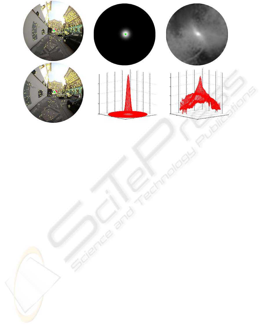
Figure 1(a) shows an easy pair which can be

solved by a standard RANSAC estimation (Hartley

and Zisserman, 2004). 57%, i.e. 1400, of tentative

matches are consistent with the true motion. Fig-

ure 1(c) shows a dominant peak in the data likelihood

p(M|e) of matches given the motion direction (Nist´er

and Engels, 2006) meaning that there is only one

motion direction which explains a large number of

matches.

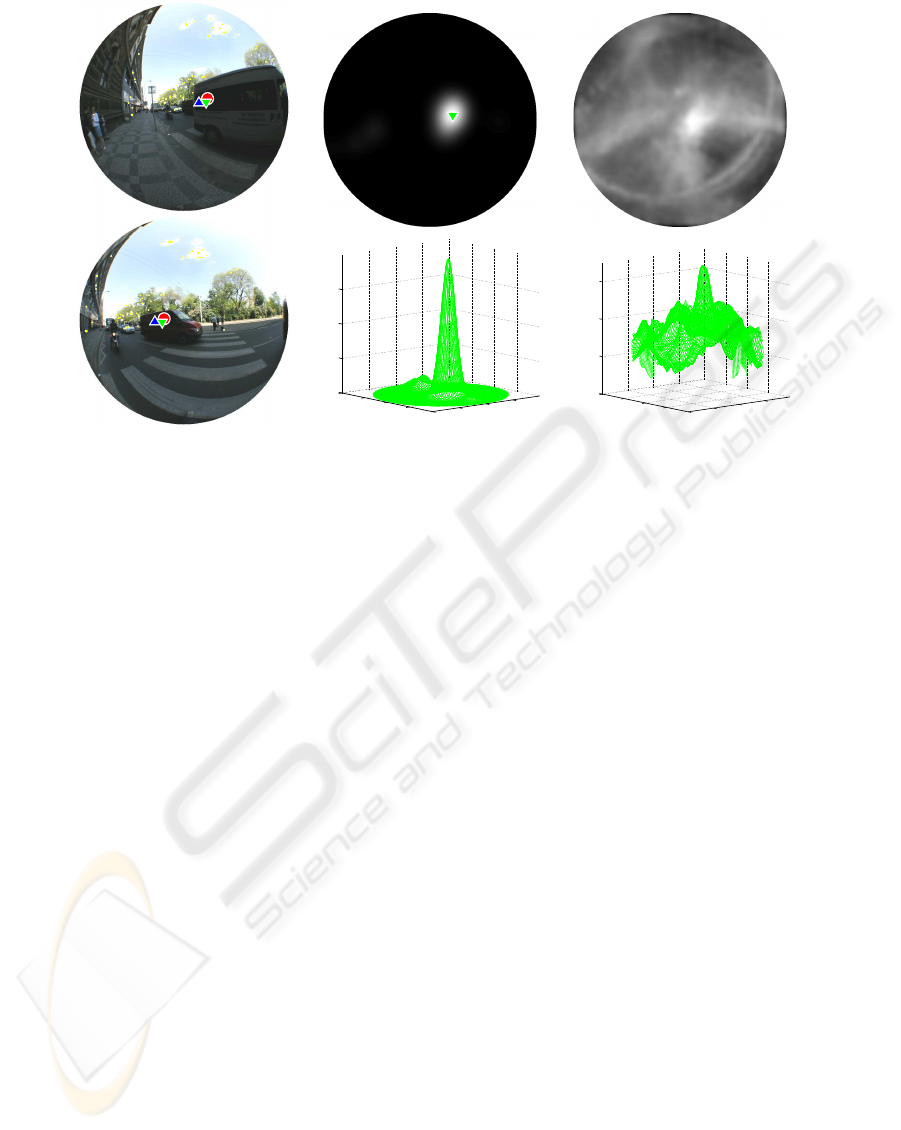
Figure 2(a) shows a more difﬁcult pair that con-

tains multiple moving objects, large camera rotation

and considerable occlusion in the scene. Only 8%,

i.e. 120, tentative matches were consistent with the

true motion. Figure 2(c) shows that there are many

577

Torii A. and Pajdla T. (2008).

OMNIDIRECTIONAL CAMERA MOTION ESTIMATION.

In Proceedings of the Third International Conference on Computer Vision Theory and Applications, pages 577-584

DOI: 10.5220/0001084505770584

 SciTePress

motion directions with high support, in this case from

wrong tentative matches.

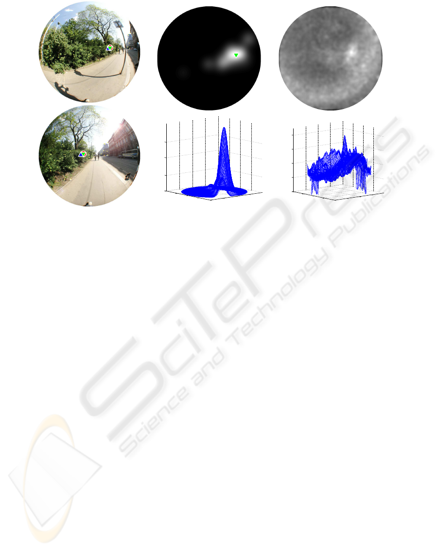
Figure 3(a) shows an even more difﬁcult pair since

only 1.4%, i.e. 50, tentative matches are consistent

with the true motion. There are very many wrong ten-

tative matches on bushes where local image features

are all small and green. Thus, many motion directions

get high support from wrong matches. The true mo-

tion has the highest support but its peak is very sharp

and thus difﬁcult to ﬁnd in limited time.

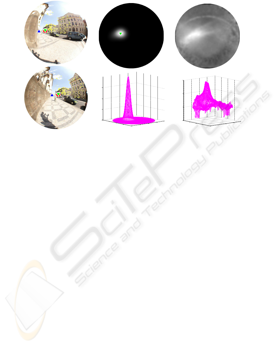
Figure. 4(a) shows a very difﬁcult pair that con-

tains large camera rotation and many repetitive fea-

tures which generate wrong tentative matches. In this

case, the motion supported by the largest number of

tentative matches is incorrect. Notice that the peak of

the likelihood of matches in Fig. 4(c) does not corre-

spond to the direction of the true motion.

All the above examples can be solved correctly by

the technique presented in this paper.

The state of the art technique for ﬁnding

relative camera orientations from image matches

ﬁrst establishes tentative matches by pairing image

points with mutually similar features and then uses

RANSAC (Fischler and Bolles, 1981; Hartley and

Zisserman, 2004; Chum and Matas, 2005) to look for

a large subset of the set of tentative matches which

is, within a predeﬁned threshold θ, consistent with

an epipolar geometry (Hartley and Zisserman, 2004).

Unfortunately, this strategy does not always recover

the epipolar geometry generated by the actual cam-

era motion. This has been observed, e.g., in (Li and

Hartley, 2005).

Often, there are more models which are supported

by a large number of matches. Thus the chance that

the correct model, even if it has the largest support,

will be found by running a single RANSAC is small.

Work (Li and Hartley, 2005) suggested to generate

models by randomized sampling as in RANSAC but

to use soft (kernel) voting for a physical parameter,

the radial distortion coefﬁcient in that case, instead

of looking for the maximal support. The best model

is then selected as the one with the parameter closest

to the maximum in the accumulator space. This strat-

egy works when the correct, or almost correct, models

met in the sampling provide consistent values of the

parameter while the incorrect models with high sup-

port generate different values of the parameter. Here

we show that this strategy works also when used for

voting in the space of motion directions.

It has been demonstrated in (Chum and Matas,

2005) that ordering the tentative matches by their

similarity may help to reduce the number of sam-

ples in RANSAC. Paper (Chum and Matas, 2005)

brought two main contributions. First, PROSAC sam-

pling strategy has been suggested which allows to uni-

formly sample from the list of tentative matches or-

dered ascendingly by the distance of their descriptors.

It allows to start by drawing promising samples ﬁrst

and often hit sufﬁciently large conﬁguration of good

matches early. The second contribution concerned a

modiﬁcation of the RANSAC stoping criterion (Hart-

ley and Zisserman, 2004, p. 119) to be able to deal

with very long sets of tentative matches without the

necessity to know their number beforehand.

When working with perspective images, it is gen-

erally accepted (Hartley and Zisserman, 2004) that

the best way to evaluate the quality of an epipolar

geometry is to look at image reprojection errors. This

is, for two images, equivalent to evaluating the dis-

tances of image points to their corresponding epipolar

lines. We compared the image reprojection error with

the residuals evaluated as the angle between rays and

their corresponding epipolar planes, which we refer

as the angular error here. In our experience, when

cameras are calibrated, the angular error can safely be

used instead of the image reprojection error. To be

absolutely correct, every ray should be accompanied

by a covariance matrix determining its uncertainty.

The matrix depends on (i) image measurement error

model and (ii) on the point position in the image. The

point position determines how the unit circle around

the point maps into the cone around the ray. In this

paper we neglected the variability of the covariance

matrix across the ﬁeld of view and assumed it to be a

scaled identity.

Next we describe how we combine ordered sam-

pling of tentative matches, soft voting, and the ori-

entation (cheirality) constraint (Hartley and Zisser-

man, 2004) on minimal ﬁve points used for comput-

ing camera motions to get an algorithm which solves

all camera motions.

2 THE ALGORITHM

Algorithm 1 presents the pseudocode of the algorithm

used to generate results described in this work. Next

we describe the key parts of the algorithm in detail.

2.1 Detecting Tentative Matches and

Computing their Descriptors

MSER (Matas et al., 2004), Harris-Afﬁne and

Hessian Afﬁne (Mikolajczyk et al., 2005) afﬁne

covariant feature regions are detected in images.

These features are alternative to popular SIFT fea-

tures (Lowe, 2004) and work comparably in our situ-

ation. Parameters of the detectors are chosen to limit

VISAPP 2008 - International Conference on Computer Vision Theory and Applications

578

(a)

0.75

0.25

0.5

(b)

0.1

0.2

0.3

0.4

0.5

(c)

Figure 1: An easy example of camera motions. (a): Fist (top) and second (bottom) images. Red ◦, blue △, and green ▽ (our

result) represent the true epipole, the epipole computed by maximizing the support, and the epipoles computed by soft voting

for the position of the epipole, respectively. Small dots show the matches giving green ▽. (b): Voting space for the motion

direction in the ﬁrst image generated by 50 soft votes casted by the result of 500-sample PROSAC, visualized on the image

plane (top) as a 3D plot (bottom). White represents large number of votes. The peak corresponds to green ▽ (our result). (c):

The maximal support for every epipole (i.e. CIF image from (Nist´er and Engels, 2006)). White represents hight support. The

image space has been uniformly sampled by 10000 epipoles and for each epipole the size of support of the best model found

by 500-sample PROSAC has been recorded.

the number of regions to 1-2 thousands per image.

The detected regions are assigned local afﬁne frames

(LAF) (Obdrˇz´alek and Matas, 2002) and transformed

into standard positions w.r.t. their LAFs. Discrete

Cosine Descriptors (Obdrˇz´alek and Matas, 2003) are

computed for each region in the standard position. Fi-

nally, mutual distances of all regions in one image

and all regions in the other image are computed as

the Euclidean distances of their descriptors and tenta-

tive matches are constructed by selecting the mutually

closest pairs.

MSER region detector is approximately 100 times

faster than the Harris and Hessian Afﬁne region de-

tector but MSERs alone were not able to solve all im-

age pairs in our data. MSERs perform great in ur-

ban environment with contrast regions, such as win-

dows, doors and markings. However, they often pro-

vide many useless regions on natural scenes because

they tend to extract contrast regions which often do

not correspond to real 3D structures, such as regions

formed by tree branches against the sky or shadows

casted by leaves.

2.2 Ordered Randomized Sampling

We use ordered sampling as suggested in (Chum and

Matas, 2005) to draw samples from tentative matches

ordered ascendingly by the distance of their descrip-

tors. We keep the original RANSAC stopping crite-

rion (Hartley and Zisserman, 2004) and we limit the

maximum number of samples to 500. We have ob-

served that pairs which could not be solved by the

ordered sampling in 500 samples got almost never

solved even after many more samples. Using the stop-

ping criterion from (Chum and Matas, 2005) often

leads to ending the sampling prematurely since the

criterion is designed to stop as soon as a large non-

random set of matches is found. Our objective is,

however, to ﬁnd a globally optimal model and not to

stop as soon as a local model with large support is

found.

We have observed that there are often several al-

ternative models with the property that the correct

model of the camera motion has a similar or only

slightly larger support than other models which are

not correct. Algorithm 1 would provide almost identi-

cal results even without the RANSAC stopping crite-

rion but the criterion helps to end simple cases sooner

OMNIDIRECTIONAL CAMERA MOTION ESTIMATION

579

(a)

0.42

0.28

0.14

(b)

0.02

0.04

0.06

0.08

(c)

Figure 2: A more difﬁcult example of camera motions. See Fig. 1.

than after 500 samples.

Having a calibrated camera, we draw 5-tuples of

tentative matches from the list M = [m]

of tentative

matches ordered ascendingly by the distance of their

descriptors. From each 5-tuple, relative orientation

is computed by solving the 5-point minimal relative

orientation problem for calibrated cameras (Nist´er,

2004; Stew´enius, 2005).

Row (sim) in Fig. 5 shows that many more cor-

rect motions have been sampled in 500 samples of

PROSAC using ordered matches than by using the

same number of samples on a randomly ordered list

of matches, row (rnd).

2.3 Orientation Constraint

An essential matrix can be decomposed into four dif-

ferent camera and point conﬁguration which differ by

the orientation of cameras and points (Hartley and

Zisserman, 2004). Without enforcing the constraint

that all points have to be observed in front of the cam-

eras, some epipolar geometries may be supported by

many matches but it need not be possible to recon-

struct all points in front of both cameras.

For omnidirectional cameras, the meaning of in-

frontness is a generalization of the classical infront-

ness for perspective cameras. With perspective cam-

eras, a point X is in front of the camera when it has a

positive z coordinate in the camera coordinate system.

For omnidirectional cameras, a point X is in front of

the camera if its coordinates can be written as a posi-

tive multiple of the direction vector which represents

the half-ray by which X has been observed.

In general, it is beneﬁcial to use only those

matches which generate points in front of cameras.

However, this takes time to verify it for all matches.

On the other hand, it is fast to verify whether the ﬁve

points in the minimal sample generating the epipolar

geometry can be reconstructed in front of both cam-

eras and to reject such epipolar geometries which do

not allow it.

Row (oc) in Fig. 5 shows that the number of incor-

rectly estimated motions decreased when such epipo-

lar geometries were excluded by this orientation con-

straint.

Furthermore, the orientation constraint in average

reduces the computational cost because it avoids eval-

uating residuals corresponding to many wrong cam-

era motions.

2.4 Soft Voting

In this paper, we vote in two-dimensional accumu-

lator for the estimated motion direction. However,

unlike in (Li and Hartley, 2005; Nist´er and Engels,

2006), we do not cast votes directly by each sampled

epipolar geometry but by the best epipolar geome-

tries recovered by ordered sampling of PROSAC.

This way the votes come only from the geometries

that have very high support. We can afford to com-

pute more, e.g. 50, epipolar geometries since the

ordered sampling is much faster than the standard

VISAPP 2008 - International Conference on Computer Vision Theory and Applications

580

(a)

0.22

0.15

0.07

(b)

0.006

0.008

0.01

0.012

0.014

(c)

Figure 3: Even more difﬁcult example of camera motions. See Fig. 1.

RANSAC. Altogether, we need to evaluate maximally

500 × 50 = 25000 samples to generate 50 soft votes,

which is comparable to running a standard 5-point

RANSAC for expected contamination by 84 % of

mismatches (Hartley and Zisserman, 2004, p. 119).

Yet, with our technique, we could go up to 98.5 %

of mismatches with comparable effort. The relative

camera orientation with the motion direction closest

to the maximum in the voting space is ﬁnally selected.

Figure 5 shows the improvementof using soft vot-

ing for ﬁnding the relative motion when casting 50

soft votes. On several difﬁcult image pairs, such as

Fig. 4, the motion supported by the largest number

of tentative matches was incorrect but the soft voting

provided a motion close to the ground truth.

3 EXPERIMENT

3.1 Image Data

Experimental data consist of 189 image pairs ob-

tained by selecting consecutive images of an image

sequence. We do not use the fact that images were

taken in a sequence and our method works for any

pair of images. The distance between two consecutive

images was 1-3 meters. Most of the camera motions

have rotations up to 15

◦

but large rotations of 45

◦

are also present. Images were acquired by Kyocera

Finecam M410R with Nikon FC-E9 ﬁsheye-lens with

183

◦

view angle. The image projection is equiangu-

lar and was internally calibrated (Miˇcuˇs´ık and Pajdla,

2006) beforehand. Images were digitized in resolu-

tion 800 pixels/183

◦

, i.e. 0.2

◦

/pixel, which is com-

parable to 240 × 180 pixels for more standard 40

◦

view angle. Acquisition of images started in a narrow

street with buildings on both sides, then continued to

a wider street with many driving cars, and ﬁnally lead

to a park with threes, bushes and walking people.

3.2 Ground Truth Motion

For most image pairs, the “true” camera motions were

recovered by running the Algorithm 1 a number of

times and checking that (i) the true motion has been

repeatedly generated by correctly matched 5-tuples

of matches and that (ii) the motion direction pointed

to the same object in both images. In a few image

pairs, for which we could not get a decisive number

of consistent results, the true motion has been gener-

ated from a 5-tuple of correct matches selected man-

ually. We estimate the precision of our ground truth

motion estimation to be higher than 4 % of the view

ﬁeld, which corresponds to 8

◦

and 32 image pixels.

3.3 Result

Figure 5(SV) shows the quality of the estimated cam-

era motion by Algorithm 1. The algorithm looks for

the motion with motion direction closest to the global

maximum in the accumulator after casting soft votes

OMNIDIRECTIONAL CAMERA MOTION ESTIMATION

581

(a)

0.52

0.34

0.17

(b)

0.04

0.07

0.1

0.13

(c)

Figure 4: A very difﬁcult example of camera motions. See Fig. 1. The motion direction with the largest support of 294

matches (b) is wrong. Our algorithm 1 ﬁnds the correct motion which is supported “only” by 287 matches.

from 50 motions. The 50 motions for soft votesare es-

timated in 500 samples by the ordered sampling based

on residuals evaluated as the angle between rays and

their corresponding epipolar planes. All motions in

our test data were estimated with motion directions

within 8

◦

, i.e. 4 % of the view angle, from the ground

truth.

4 CONCLUSIONS

We have presented a practical algorithm which can

compute camera motions from omnidirectional im-

ages. We have improved the state of the art by com-

bining ordered sampling from tentative matches or-

dered by their descriptor similarity with the orienta-

tion constraintand soft voting. We used angular resid-

ual error which better ﬁts to the geometry of omni-

directional cameras. Our algorithm was able to cor-

rectly compute motions of all tested 189 image pairs.

ACKNOWLEDGEMENTS

The authors were supported by EC project FP6-IST-

027787 DIRAC and by Czech Government under the

reseach program MSM6840770038. Any opinions

expressed in this paper do not necessarily reﬂect the

views of the European Community. The Community

is not liable for any use that may be made of the in-

formation contained herein.

REFERENCES

2d3 Ltd. Boujou. http://www.2d3.com.

Brown, M. and Lowe, D. G. (2003). Recognising panora-

mas. In ICCV ’03, Washington, DC, USA.

Chum, O. and Matas, J. (2005). Matching with PROSAC

- progressive sample consensus. In CVPR ’05, vol-

ume 1, pages 220–226, Los Alamitos, USA.

Cornelis, N., Cornelis, K., and Gool, L. V. (2006).

Fast compact city modeling for navigation pre-

visualization. In CVPR ’06, pages 1339–1344, Wash-

ington, DC, USA.

Davison, A. J. and Molton, N. D. (2007). Monoslam: Real-

time single camera slam. IEEE Transactions on Pat-

tern Analysis and Machine Intelligence, 29(6):1052–

1067.

Fischler, M. A. and Bolles, R. C. (1981). Random sample

consensus: a paradigm for model ﬁtting with appli-

cations to image analysis and automated cartography.

Commun. ACM, 24(6):381–395.

Hartley, R. I. and Zisserman, A. (2004). Multiple View

Geometry in Computer Vision. Cambridge University

Press, ISBN: 0521540518, second edition.

Li, H. and Hartley, R. (2005). A non-iterative method for

correcting lens distortion from nine point correspon-

dences. In OMNIVIS ’05.

VISAPP 2008 - International Conference on Computer Vision Theory and Applications

582

20 40 60 80 100 120 140 160 180

rnd

sim

Image number

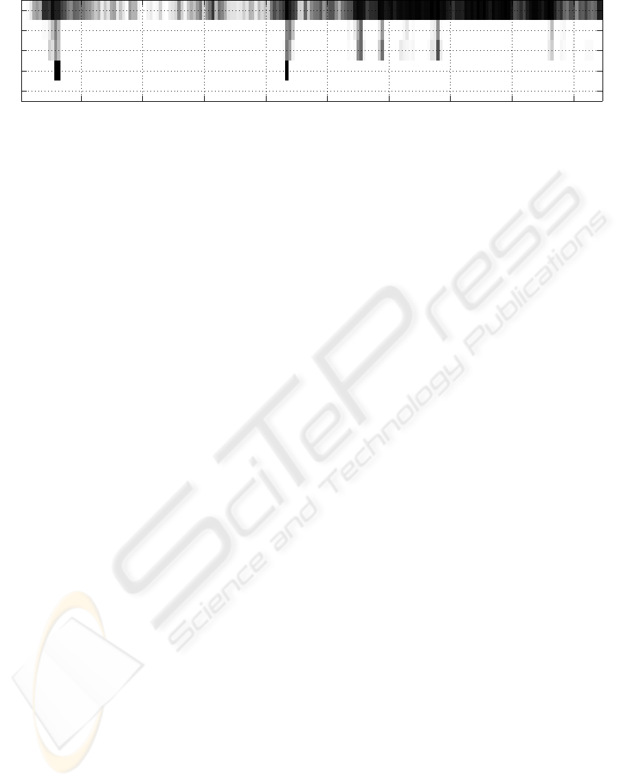
Figure 5: Camera motion estimation obtained by the ordered sampling, orientation constraint, and soft voting. The graph

shows the number of camera motion directions that are not further than 8

◦

from the ground truth as a function of the image

pair (i,i + 1) with i on the horizontal axis. Lighter color represents higher numbers. The motion directions were computed

from the ﬁrst 500 5-point samples drawn from tentative matches ordered randomly, row (rnd), and tentative matches ordered

by their similarity, row (sim). Ordering of tentative matches by similarity greatly increased the number of correctly estimated

epipoles. Row (oc) shows the number of epipolar geometries for which the 5 points of their generating minimal sample get

reconstructed in front of both cameras (orientation constraint). Using the orientation constraint further improves the result.

Row (MS) shows whether the motion direction, which is supported by the largest number of tentative matches in 50 motions,

is (black) or is not (white) more than 8

◦

apart from the true motion direction. Row (SV) shows whether the estimated motion

direction, which is closest to the global maximum in the accumulator, is (black) or is not (white) more than 8

◦

apart from the

true motion direction. This is the best strategy for estimating the camera motion.

Lowe, D. G. (2004). Distinctive image features from scale-

invariant keypoints. International Journal of Com-

puter Vision, 60(2):91–110.

Martinec, D. and Pajdla, T. (2007). Robust rotation and

translation estimation in multiview reconstruction. In

CVPR ’07, Minneapolis, MN, USA.

Matas, J., Chum, O., Urban, M., and Pajdla, T. (2004).

Robust wide-baseline stereo from maximally stable

extremal regions. Image and Vision Computing,

22(10):761–767.

Miˇcuˇs´ık, B. and Pajdla, T. (2006). Structure from motion

with wide circular ﬁeld of view cameras. IEEE Trans-

actions on Pattern Analysis and Machine Intelligence,

28(7):1135–1149.

Mikolajczyk, K., Tuytelaars, T., Schmid, C., Zisserman, A.,

Matas, J., Schaffalitzky, F., Kadir, T., and Gool, L. V.

(2005). A comparison of afﬁne region detectors. Inter-

national Journal of Computer Vision, 65(1-2):43–72.

Nist´er, D. (2004). An efﬁcient solution to the ﬁve-point

relative pose problem. IEEE Transactions on Pattern

Analysis and Machine Intelligence, 26(6):756–777.

Nist´er, D. and Engels, C. (2006). Estimating global un-

certainty in epipoloar geometry for vehicle-mounted

cameras. In SPIE, Unmanned Systems Technology

VIII, volume 6230.

Obdrˇz´alek,

S. and Matas, J. (2002). Object recognition us-

ing local afﬁne frames on distinguished regions. In

BMVC ’02, volume 1, pages 113–122, London, UK.

Obdrˇz´alek,

S. and Matas, J. (2003). Image retrieval us-

ing local compact dct-based representation. In DAGM

’03, number 2781 in LNCS, pages 490–497, Berlin,

Germany.

Pritchett, P. and Zisserman, A. (1998). Wide baseline stereo

matching. In ICCV ’98, pages 754–760, Bombay, In-

dia.

Schaffalitzky, F. and Zisserman, A. (2001). Viewpoint in-

variant texture matching and wide baseline stereo. In

ICCV ’01, Vancouver, Canada.

Stew´enius, H. (2005). Gr¨obner Basis Methods for Minimal

Problems in Computer Vision. PhD thesis, Centre for

Mathematical Sciences LTH, Lund University, Swe-

den.

Tuytelaars, T. and Gool, L. V. (2000). Wide baseline stereo

matching based on local, afﬁnely invariant regions. In

BMVC ’00, Bristol, UK.

Williams, B., Klein, G., and Reid, I. (2007). Real-time slam

relocalisation. In ICCV ’07, Rio de Janeiro, Brazil.

OMNIDIRECTIONAL CAMERA MOTION ESTIMATION

583

Algorithm 1 Camera motion estimation by orderedsampling from tentative matches with geometricalconstraints.

Input: Image pair I

, I

θ := 0.3

◦

.. .the tolerance for establishing matches

σ := 4

◦

.. .the standard deviation of Gaussian kernel for soft voting

:= 50 ...the number of soft votes

:= 500 ...the maximum number of random samples.

η := 0.95 .. .the termination probability of the standard RANSAC (Hartley and Zisserman, 2004, p. 119).

Output: Essential matrix E

∗

1. Detect tentative matches and compute their descriptors.

1.1 Detect afﬁne covariant feature regions MSER-INT+, MSER-INT-, MSER-SAT+,

MSER-SAT-, APTS-LAP, and APTS-HES in left and right images, Sec. 2.1.

1.2 Assign local afﬁne frames (LAF) (Obdrˇz´alek and Matas, 2002) to the regions and transform the regions

into a standard position w.r.t. their LAFs.

1.3 ComputeDiscrete Cosine Descriptors (Obdrˇz´alek and Matas, 2003) for each region in the standardposition.

2. Construct the list M = [m]

of tentative matches with mutually closest descriptors. Order the list ascendingly

by the distance of the descriptors. N is the length of the list.

3. Find a camera motion consistent with a large number of tentative matches:

1: Set D to zero. // Initialize the accumulator of camera translation directions.

2: for i := 1,...,N

3: t := 0 // The counter of samples. n := 5 // Initial segment length.

:= N

// Initial termination length.

4: while t ≤ N

5: if t = ⌈200000









⌉ (Chum and Matas, 2005) then

6: n := n + 1 // The maximum number of samples for the current initial segment reached, increase

the initial segment length.

7: end if

8: t := t + 1 // New sample

9: Select the 5 tentative matches M

of the t

sample by taking 4 tentative matches from [m]

n−1

random and adding the 5

match m

10: E

:= the essential matrix by solving the 5-point minimal problem for M

(Nist´er, 2004; Stew´enius,

2005).

11: if M

can be reconstructed in front of cameras (Hartley and Zisserman, 2004, p. 260) then

12: S

:= the number of matches which are consistent with E

, i.e. the number of all matches m =

] for which max(∡(u

),∡(u

⊤

)) < θ.

13: else

14: S

:= 0

15: end if

16: N

:= log(η)/log



1−











//The termination length deﬁned by the maximality con-

straint (Hartley and Zisserman, 2004, p. 119).

17: N

:= min(N

) // Update the termination length.

18: end while

19:

t = arg

t=1,...,N

maxS

// The index of the sample with the highest support.

20:

:= E

:= camera motion direction for the essential matrix E

21: Vote in accumulator D by the Gaussian with sigma σ and mean at

22: end for

23:

e := arg

x∈domain(D)

maxD(x) // Maximum in the accumulator.

24: i

∗

:= arg

i=1,...,50

min∡(

) // The motion closest to the maximum.

25: E

∗

// The “best” camera motion.

4. Return E

∗

VISAPP 2008 - International Conference on Computer Vision Theory and Applications

584