ACTIVE APPEARANCE MODEL (AAM)

From Theory to Implementation

Nikzad Babaii Rizvandi, Aleksandra Piˇzurica and Wilfried Philips

Image Processing and Interpretation Group (IPI), Department of Telecommunications and Information Processing (TELIN)

Gent University, St-Pietersnieuwstraat 41, B-9000 Gent, Belgium

Keywords:

Shape Model, Texture Model, Active Appearance Model, Active Shape model, advantages and disadvantages.

Abstract:

Active Appearance Model (AAM) is a kind of deformable shape descriptors which is widely used in computer

vision and computer graphics. This approach utilizes statistical model obtained from some images in training

set and gray-value information of the texture to ﬁt on the boundaries of a new image. In this paper, we describe

a brief implementation, apply the method on hand object and ﬁnally discuss its performance in compare to

Active Shape Model(ASM). Our experiments shows this method is more sensitive to the initialization and

slower than ASM.

1 INTRODUCTION

Model-based approaches analyze different variations

of an object using some samples of the object in a

training set and ﬁnally calculate a model based on the

object variations. Active Appearance Model (AAM)

of Cootes et al. in (T.F.Cootes and C.J.Taylor, 2001)

is one of the well-known model-based methods.

To build an AAM model, a training set of images

is assumed in which corresponding landmark points

have been marked on every image. A statistical model

of the shape variation by using these landmarks and

Principle Component Analysis (PCA), a model of the

texture variation (sampling of the gray values of im-

ages) using mean shape, delaunay triangles and an-

other PCA and a model of the correlations between

shape and texture, are computed. The ﬁnal shape-

texture model and the images in the training set are a

basis to learn a multi-variate regression matrix. With

enough training examples this model should be able

to synthesize any image of normal anatomy. By ﬁnd-

ing the parameters which optimize the match between

a synthesized model image and a target image all the

structures represented by the model can be located.

Obtaining a model by AAM includes two main stages

which are:

• Ofﬂine stage:

- Manual Labeling: Placing landmarks surround-

ing objects in images inside training set manually.

(T.F.Cootes and J.Graham, 1995) explains differ-

ent kinds of landmarks.

- Shape Alignment: The differences among

shapes, which are rotation, x-y translations and

scaling, are omitted and mean shape is created.

- Statistical Shape Model: using PCA the aligned

shape variations are modeled as an eigenvector

matrix and a few parameters.

- Texture Sampling: The gray-value of each pixel

under each shape in the training set is obtained.

- Texture Alignment: Texture alignment is used in

order to omit the illumination differences among

the images in the training set.

- Statistical Texture Model:After texture align-

ment another PCA is utilized to model the typical

texture variations.

- Joint Shape-Texture Statistical Model: Both

shape and texture models are merged together to

construct an unit model.

- Training Regression Matrix: A multivariate lin-

ear regression matrix is trained using the joint

model and some images in the training set.

• Online stage:

- Search in a New Image: The obtained AAM

model along with the regression matrix are used

to ﬁnd the modeled object in a new image.

539

Babaii Rizvandi N., Pižurica A. and Philips W. (2008).

ACTIVE APPEARANCE MODEL (AAM) - From Theory to Implementation.

In Proceedings of the Third International Conference on Computer Vision Theory and Applications, pages 539-542

DOI: 10.5220/0001081705390542

 SciTePress

In this paper, we describe a brief implementation

of AAM, then we examine AAM on hand object

and ﬁnally compare AAM performance with another

model-based method named Active Shape Model

(ASM).

2 OFFLINE STAGE

This stage utilizes some statistical analysis by using

Principle Component Analysis (PCA) on the shape

variations and also texture variations of some gath-

ered images in a training set.

2.1 Manual Labeling

In the analyzed model, the shape is represented by

a set of points (or landmarks). These landmarks

are placed manually for each shape in the training

set. The corresponding landmarks in the shapes must

be approximately in the same location because each

point represents a particular part of the object or

its boundary. To increase accuracy some additional

points are added between two points when the dis-

tance is more than a threshold.

2.2 Shape Alignment

All objects in the training set has different scaling,

rotation and x-y position(or translation), named pose

parameters, compare to the others. In order to re-

move the pose differences and only remain the object

shape variations the alignment procedure is used. The

center of mass of the shape is calculated and moved

to the coordinate origin for removing X-Y transla-

tion. After removing the X-Y translation the obtained

shape becomes unity scale by dividing the shape on

its L

− norm. To remove the rotation, another shape

is needed as a reference. It can be proved mathe-

matically that Singular Value Decomposition (SVD)

calculates the rotation matrix between the shape and

the reference shape. A comprehensive explanation of

shape alignment with its procedure can be found in

(Babaii Rizvandi et al., 2007). The mentioned proce-

dure is only for one shape. For the shapes in the train-

ing set, we align all shapes to the ﬁrst shape and cal-

culate the mean shape. Then we align all shapes to the

mean shape and we recalculate the mean shape. This

procedure, which aligns to the mean shape and recal-

culates the mean shape, is continued until the mean

shape does not change signiﬁcantly in two iterations.

2.3 Statistical Shape Model

The 2N elements are highly correlated, so it is possi-

ble to represent them much more compactly. One ap-

proach is Principle Component Analysis (PCA) that

is widely used in pattern recognition to reduce the di-

mension. Using PCA the number of elements reduces

from 2N to M while M << 2N. The ﬁnal shape model

X = X + Φ

shape

(1)

where X is the mean shape, Φ

shape

contains the shape

eigenvectors and b

shape

includes the shape parame-

ters.

2.4 Texture Sampling

The question to make a texture model is which gray

values must be used in the model and how the model

should be deﬁned. The answer to the ﬁrst question

is that only pixels including the object are necessary.

Dividing the shape into a combination of triangles by

delaunay triangulation is the common solution for the

second question.

The problem with delaunay triangulation is that

these triangles cover all regions including background

of the convex hull (Stegmann, 2000), (T.F.Cootes and

J.Graham, 1995). So in order to form a suitable tex-

ture model, a convex hull algorithm must be used.

After removing the background pixels, the next

step is to ﬁnd the corresponding pixels in the object

textures and warp these pixels positions. To do this

task, the pixels inside the mean shape are sampled

and the related pixels in the other images textures in

the training set are obtained by using the correspond-

ing triangles. (Stegmann, 2000) and (Babaii Rizvandi

et al., 2007) explain the complete algorithm.

2.5 Texture Alignment

Within the object there are usually some variations

in gray values because of different illumination in-

tensities. Since the goal is to build a stable model

without these unwanted effects, these variations must

be eliminated. The common method is to align all

textures to the standardized mean texture, with zero

mean and unit variance, and continue this procedure

till the difference between the standardized mean tex-

ture in two following iterations is less than a threshold

[(T.F.Cootes and C.J.Taylor, 2001) ,(Stegmann, 2000)

and (Babaii Rizvandi et al., 2007)].

VISAPP 2008 - International Conference on Computer Vision Theory and Applications

540

2.6 Statistical Texture Model

The same as section 2.3 another PCA is used to rep-

resent the obtained texture information much more

compactly. Because the number of elements in the

texture is much higher, using the traditional PCA

takes a lot of time. If N

and N are the number of

texture pixels and the number of shapes in the train-

ing set, so the covariance matrix will have N

∗ N

dimensions. When N

≫ N, calculating the covari-

ance matrix, and therefore the texture eigenvectors

and eigenvalues, is computationally expensive. The

idea is to calculate the covariance between the tex-

tures and then convert it to the covariance between

the pixels (Stegmann, 2000). The ﬁnal texture model

T = T +Φ

tex

(2)

where T is the mean texture, Φ

tex

contains the texture

eigenvectors and b

tex

includes the texture parameters.

2.7 Joint Shape-Texture Model

Both b

shape

and b

tex

models should be merged to form

a unit model including both texture and shape vari-

abilities and keeping the correlation between them.

Since the nature of shape and texture are different,

some weighting is necessary. In the absence of these

weighting, spread of the points in the space will be

undesirable (Stegmann, 2000). A simple weighting

matrix is a diagonal matrix:

W = wI =





w · ·· 0

0 · · · w





(3)

where w =

Σλ

tex

Σλ

shape

and λ

tex

and λ

shape

are eigenval-

ues of b

shape

and b

tex

, respectively. The merged model

is a simple column vector:

joint



W ∗ b

shape

tex



(4)

To eliminate correlation between shape and tex-

ture parameters, another PCA should be performed

on the combined data (b

joint

= φ

joint

∗ c (5)

where φ

joint

is the eigenvector matrix of joint shape-

texture parameters and c is the ﬁnal combined model

parameters. The same as the section 2.3, the order of

model is reduced after calculating the PCA.

The ﬁnal shape and texture models are calcu-

lated with the following equations (T.F.Cootes and

C.J.Taylor, 2001), (Zambal, 2005):

X = X + φ

shape

∗ W

−1

∗ φ

joint,shape

∗ c

T = T + φ

tex

∗ φ

joint,tex

∗ c (6)

where

joint



joint,shape

joint,tex



(7)

These two equations are the basis to calculate the re-

gression matrix in the next level.

2.8 Training a Regression Matrix

The search procedure in AAM is considered as an

optimization problem in which the gray value differ-

ences between the artiﬁcial object obtained by AAM

and an actual image is to be minimized:

δI = I

image

− I

model

(8)

In this case the optimization can be enhanced by ad-

justing the model and pose parameters in order to ﬁt

the artiﬁcial object with the image. So δI can be re-

placed by δT because this procedure is based on the

normalized texture vectors (Stegmann, 2000). One

possibility is that to consider the relation between δT

and the model-pose parameters changes, δc, as lin-

ear and use the information obtained from the joint

shape-texture model and the texture of some images

in the training set in a linear regression matrix (R) as

following:

´c

= Rδ

(9)

where ´c = [c,t

, θ, S]. The idea of the standard

AAM approach is to estimate R in a precalculation

step. The parameters of a model instance are changed

and the according differences in texture are measured.

If the parameter differences are the column vectors of

a second matrix ∆

´c

and each of ∆

represents the tex-

ture differences corresponding to the parameters dif-

ferences, the last equation becomes

∆

´c

= R∆

(10)

The ﬁnal R can be calculated as (Zambal, 2005)

R = ∆

´c

ΦΛ

−1

∆

(11)

where Λ and Φ are eigenvalues and eigenvectors for

matrix ∆

∆

´c

, respectively.

3 ONLINE STAGE

In the online stage, we use the constructed AAM

model in order to ﬁt the model on a target object in

a new image. The following is the standard AAM

search algorithm (T.F.Cootes and C.J.Taylor, 2001)

and (Zambal, 2005).

- Place an initial shape near the desired object in the

new image.

ACTIVE APPEARANCE MODEL(AAM) - From Theory to Implementation

541

• Repeat

- Calculate the texture differences δ

- Calculate the parameter differences by using

´c

= Rδ

- ´c → ´c+ δ

´c

- Calculate the differences between artiﬁcial

model texture and image texture belong the arti-

ﬁcial model shape(E).

• until E ≤ Threshold

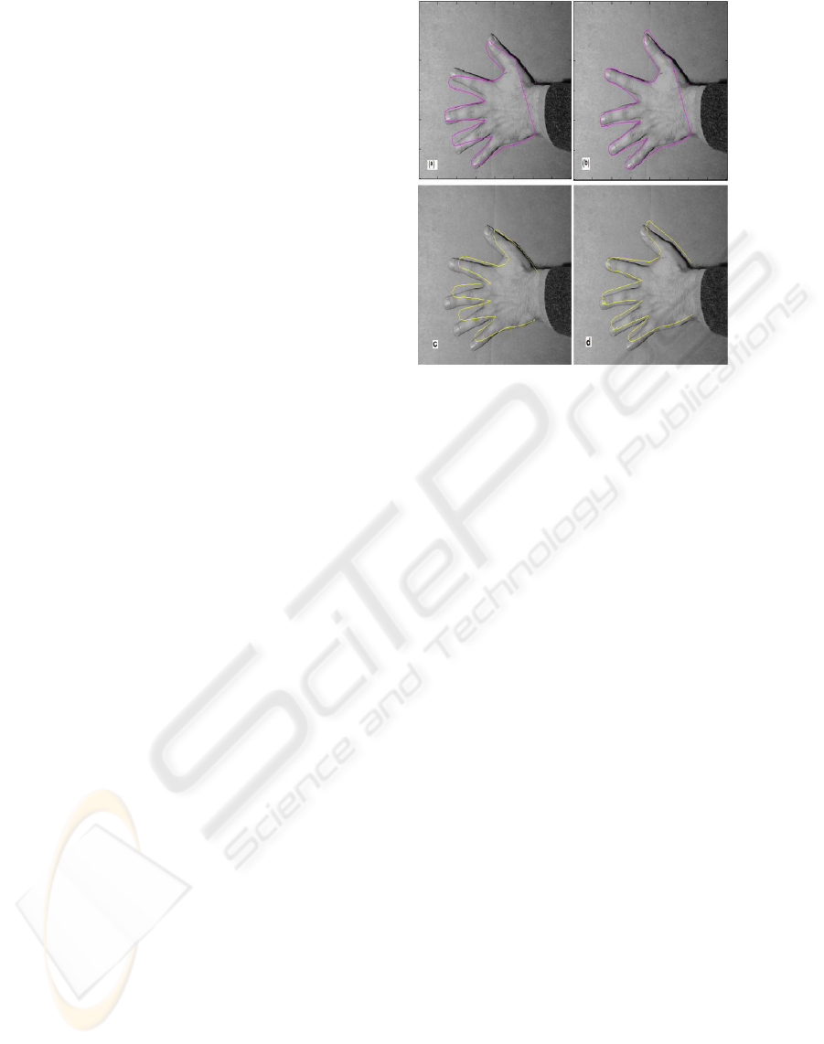
4 EXPERIMENTAL RESULTS

Hand Gesture Extraction is one of the common appli-

cations of Active Appearance Model (AAM) and Ac-

tive Shape Model (ASM). In this section, we applied

our implementation of Active Appearance Model

(AAM) and Active Shape Model (ASM) on images

of hand in order to compare these method efﬁcien-

cies. At ﬁrst the images of hand must be labeled with

some landmarks. In our implementation both AAM

and ASM iterate 40 times. Figure.1 shows the result

of both AAM and ASM for a suitable initialization.

Our experiment shows the efﬁciency of both methods

has an extreme dependence on two factors: (a) com-

prehensive object variations in the training set that

means all changes outside of the training set are not

included by the model and (b) a suitable initialization.

ASM searches around the current location so it has

a larger capture range than the AAM which only con-

siders the image directly under its current area. ASM

only uses data around the model landmarks and does

not involve all the grey-level information available

across an object as the AAM does. Thus it may be

less reliable. In compare to AAM, ASM is faster and

achieves more accurate feature point location than the

AAM, but tends to be less reliable.

5 CONCLUSIONS

In this paper, we examined the AAM model perfor-

mance for ﬁnding the boundary of hand. We also

compared its efﬁciency with another deformable

method named Active shape model (ASM). The re-

sults show that because this method uses gray-values

information of images, it is slower than the ASM.

Moreover, due to using the local information its

capture range is less than ASM and so more sensitive

to the initialization than ASM.

Figure 1: Experimental results for AAM in compare to

ASM: (a) initial shape for ASM (b) Final Shape for ASM

ACKNOWLEDGEMENTS

The author N.Babaii Rizvandi is supported as a Re-

search Assistant by Gent University under doctoral

grant. A.Piˇzurica is a postdoctoral research fellow of

FWO, Flanders.

REFERENCES

Babaii Rizvandi, N., Philips, W., and Pizurica, A. (2007).

Active appearance model construction: Implementa-

tion notes. In Proc. 10th Joint Conference on Infor-

mation Sciences, Salt Lake City, USA. 7 pages.

Stegmann, M. B. (2000). Master thesis. In Active Appear-

ance Models: Theory, Extensions and Cases. Techni-

cal university of Denmark.

T.F.Cootes, C.J.Taylor, D. and J.Graham (1995). In Active

Shape Models: Their Training and Application. Com-

puter Vision and Image Understanding.

T.F.Cootes, G. and C.J.Taylor (June 2001). In Active ap-

pearance Models. IEEE Transactions on Pattern Anal-

ysis and Machine Intelligence.

Zambal, S. (August 2005). Master thesis. In 3D Active

Appearance Models for segmentation of Cardiac MRI

data. Technische Universitat Wien, Austria.

VISAPP 2008 - International Conference on Computer Vision Theory and Applications

542