DETECTING, TRACKING AND COUNTING FISH IN LOW

QUALITY UNCONSTRAINED UNDERWATER VIDEOS

Concetto Spampinato

Department of Informatics and Telecommunication Engineering, University of Catania, Catania, Italy

Yun-Heh Chen-Burger, Gayathri Nadarajan and Robert B. Fisher

School of Informatics, University of Edinburgh, Edinburgh, UK

Keywords: Motion detection, Tracking, Fish image processing, Under-water marine life observation.

Abstract: In this work a machine vision system capable of analysing underwater videos for detecting, tracking and

counting fish is presented. The real-time videos, collected near the Ken-Ding sub-tropical coral reef waters

are managed by EcoGrid, Taiwan and are barely analysed by marine biologists. The video processing

system consists of three subsystems: the video texture analysis, fish detection and tracking modules. Fish

detection is based on two algorithms computed independently, whose results are combined in order to

obtain a more accurate outcome. The tracking was carried out by the application of the CamShift algorithm

that enables the tracking of objects whose numbers may vary over time. Unlike existing fish-counting

methods, our approach provides a reliable method in which the fish number is computed in unconstrained

environments and under several scenarios (murky water, algae on camera lens, moving plants, low contrast,

etc.). The proposed approach was tested with 20 underwater videos, achieving an overall accuracy as high

as 85%.

1 INTRODUCTION

Traditionally, marine biologists determine the

existence and quantities of different types of fish

using several methods, including casting nets in the

ocean for collecting and examining fish, human

underwater observation and photography (Rouse

2007, Schlieper 1972), combined net casting and

acoustic (sonar) (Brehmera et. al, 2006) and, more

recently, human hand-held video filming.

Each of such methods has their drawbacks. For

instance, although the net-casting method is

accurate, it kills the collected fish, damages their

habitat and costs much time and resources. Human

manned photography and video-making but do not

damage observed fish or their habitat, the collected

samples are scarce or limited and is intrusive to the

observed environment therefore do not capture

normal fish behaviours.

This paper presents an alternative approach by

using an automated Video Processing (VP) system

that analyses videos to identify interesting features.

These videos are taken automatically and

continuously by underwater video-surveillance

cameras near the Ken-Ding Taiwan sub-tropical

coral reef waters. The video collection was produced

as a part of the on-going efforts of the Taiwanese

EcoGrid project (http://ecogrid.nchc.org.tw).

The proposed automated video processing

system is able to handle large amount of videos

automatically and speedily gives those un-watched

video clips a chance to be analysed. The system’s

performance is promising, as shall be reported later

on in this paper.

The challenges that differentiate the undertaken

work as reported here when compared with other

traditional methods are in the nature of the videos to

be processed. Traditionally, such tasks only deal

with videos taken in a controlled environment or a

lab, e.g. a fish tank with fixed lighting, cameras,

background, fixed objects in the water, known types

of fish, etc. Based on these pre-determined

conditions, the VP software can be gradually tuned

to suit this fixed environment and gains better

performance over time.

This condition, however, was not possible in our

case, as our videos were taken in an un-controlled

open sea where the degree of luminosity and water

flow may vary depending upon the weather and the

time of the day. The water may also have varying

degrees of clearness and cleanness. Moreover,

unlike a normal fish tank in a lab, open sea videos

will consist of “non-fish” moving objects – which

514

Spampinato C., Chen-Burger Y., Nadarajan G. and B. Fisher R. (2008).

DETECTING, TRACKING AND COUNTING FISH IN LOW QUALITY UNCONSTRAINED UNDERWATER VIDEOS.

In Proceedings of the Third International Conference on Computer Vision Theory and Applications, pages 514-519

DOI: 10.5220/0001077705140519

 SciTePress

require additional handling to eliminate. In addition,

as algae grow rapidly in subtropical waters and on

camera lens, it affects the quality of the videos

taken. Consequently, different degrees of greenish

and bluish videos are produced. In order to decrease

the algae, frequent and manual cleaning of the lens

is required.

The next session introduces our three Image

Processing (IP) Tasks, which is followed by a

description of our texture and colour analysis

subsystem. The fish detection and tracking systems

are then described followed by an analysis of their

performance. We report an 85.72% overall success

rate over 20 movies (about 8000 frames) when

comparing with a current state of the art, e.g in

(Morais et al, 2005) 81% success rate, that operates

on video clips shot in a controlled environment.

2 IMAGE PROCESSING TASKS

Currently, marine biologists manually analyse

underwater videos to find useful information. This

procedure requires a lot of time and human

concentration, as an operational camera will

generate imagery data of about 2 Terabytes (20

millions frames) per year. Moreover, most of such

analyses are done un-aided by VP/IP software. For

one minute’s video, it will take a human about 15

minutes for classification and annotation. To fully

analyse existing videos alone, generated by the three

underwater cameras over the past four years, will

take human approximately 180 years.

The proposed system therefore aims to support

the non-VP trained users to leverage VP and IP

software to help their normal line of work.

Given an underwater video, our system analyses

it and provides relevant information, e.g. the number

of fish present, quality of the video (clear, murky,

smoothed, etc), dominant colour of the video. To

provide such information, the developed video

processing system consists of three main image

processing subsystems: Texture and Colour

Analysis, Fish Detection, and Fish Tracking.

The output of our VP system is provided both by

displaying the coarse-grained results directly onto

the video and in elaborated, ontologically grounded

Prolog predicates in a text file.

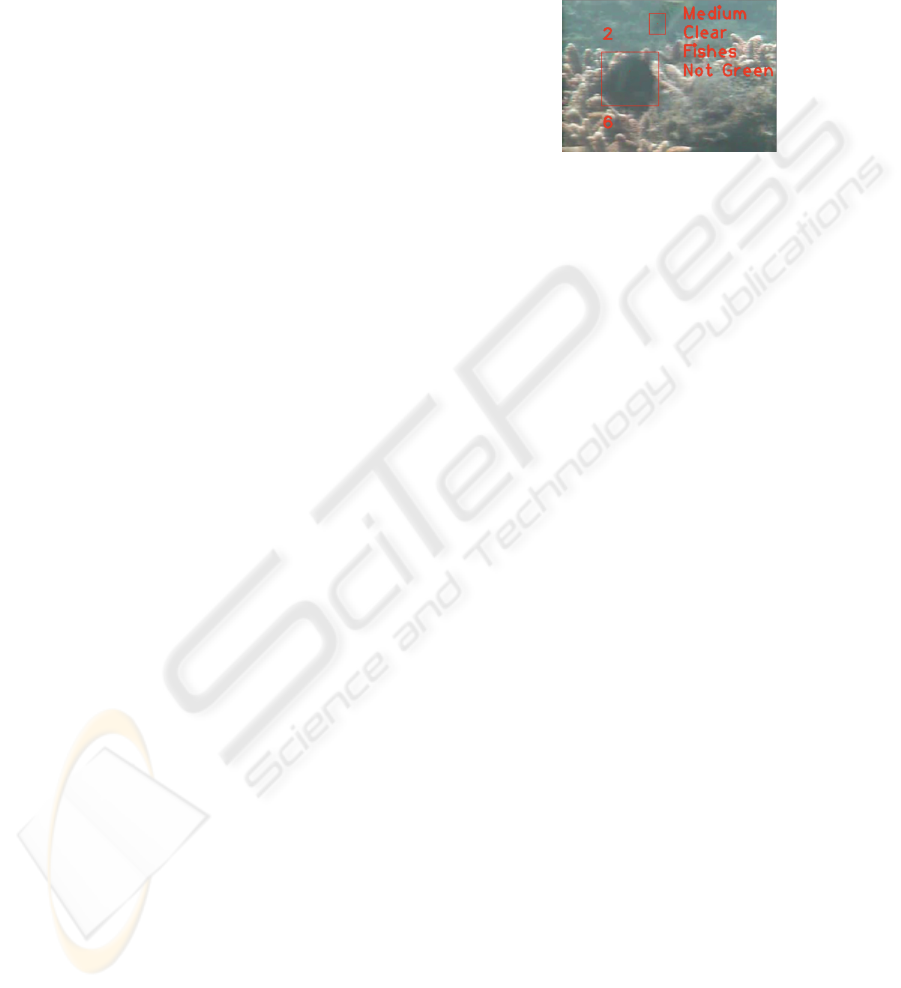
Figure 1 illustrates the classification information

generated by the system as displayed in a video:

Medium, Clear, Fishes, Not Green. They represent

the average luminosity, the average smoothness, the

presence (or non-presence) of fish and the green-

toned quality of the frame. The top left number (2)

indicates the numbers of fish in the frame and the

lower left number (6) indicates the total numbers of

fish in the whole video. The two square boxes

surround fish identified by the system. Most of the

annotations are given in plain natural language

(medium, clear, etc) for a better understanding for

non-image processing people like the marine

biologists.

Figure 1: Annotations as displayed in a processed video.

3 TEXTURE AND COLOUR

ANALYSIS SYSTEM

The aim of this subsystem is to detect the average

texture and colour properties of each frame. The

evaluated properties are: 1) Brightness: classified in

Dark/Medium/ Bright; 2) Smoothness: classified in

Blur/Clear; 3) Colour: identification of green colour

tone, classified in Green/Not Green; Hue,

Saturation and Value: classified in

High/Medium/Low.

The approach used for describing the image

texture (e.g. brightness and smoothness) is based on

analysing the statistical moments of the grey-level

histogram. Let z be a random variable denoting

image grey levels and p(z

) i=1,2, …., L-1 be the

corresponding histogram, here L represents the

distinct grey levels. p(z

), i=1…N is the normalized

histogram, so that

1)(

∑

The n

moment of the grey level histogram of an

image is therefore:

(z) = (z

− m)

⋅ p(z

)

−

∑

(1)

∑

−

⋅=

)()(

zpzm

Where m is the mean value of z (the average grey

level). The variance is the second order momentum

. The third order moment μ

is a measure of the

skewness of the histogram, while the fourth order

moment μ

is a measure of its relative flatness.

Other measures that we use are the uniformity U

and the entropy E:

U = p

)

−

∑

(2)

E =− p(z

) ⋅log

p(z

)

i= 0

L−1

∑

(3)

DETECTING ,TRACKING AND COUNTING FISH IN LOW QUALITY UNCONSTRAINED UNDERWATER

VIDEOS

515

In particular, for constant images U =1 and E= 0.

Using these values, we can estimate the brightness

(formula 4) and the smoothness (formula 5)

characteristics.

bright

=m +

(z) ⋅ 255

(4)

smooth

⋅

⎟

⎠

⎞

⎜

⎝

⎛

++=

)(

μμ

(5)

Where k is constant, usually set to 10. If r

bright

a video is found to be larger than a pre-determined

threshold, we classify this video as “Bright”.

Similarly, we use r

smooth

and its corresponding

threshold to determine the smoothness of a video.

For colour analysis, we extract the Hue, Saturation

and Value planes. For each plane, we compute the

averaged percentage of the pixels whose value is

larger than a suitable threshold in the video.

To determine whether a video is Green colour

toned or not, we determine the green plane of a

frame and then we count all the pixels in such plane

which value is greater than 128. Nextly we

aggregate those values to decide the overall green

colour tone of the video. These results are stored in

relevant Prolog predicates.

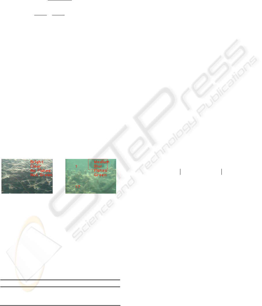
Sample images of real videos captured in the sea

are provided in Figure 2, with the machine-

generated annotation displayed on them.

(a)

(b)

Figure 2: Example classified video results.

The classification task was done on all 20 videos,

using the texture and colour analysis subsystem.

Table 1 shows the obtained results for the texture

analysis, where NV indicates the number of videos

that weren’t correctly classified, PV the number of

videos correctly classified and CSR the success rate

for each analysed feature.

Table 1: Classification Results.

Feature NV PV % CSR

Smoothness 1 19 95%

Brighteness 1 19 95%

Colour 2 18 90%

4 FISH DETECTION SYSTEM

One piece of useful information for marine

biologists is the number of fish present in a video,

which can help them identify promising videos.

Object detection is therefore needed.

The main difficulty encountered was the choice

of the fish detection algorithm, which has the

fundamental influence on the performance of the

tracking and counting systems. Given the main

constraint of fast processing over the large amount

of video data, most of the algorithms explored were

based on subtracting a reference image, representing

the background, from the current input image.

Before selecting the moving average algorithm,

we considered several algorithms (the Gaussian

Model (Rajagopalan et al, 1999) and the H-Model

(Faro et. al., 2004) that avoided the computationally

expensive background updating step, based on the

use of morphological and spatial filters.

The main shortcoming of these algorithms were

the large processing time and the difficulty of

choosing a generally applicable sequence of filters

and parameters. Therefore, a moving average

algorithm was selected, because it gave a good

balance between processing time and accuracy over

the static scenarios.

So let CB and FR

be background image and n

frame, respectively. Then the moving pixels of

frame n, MP

, are detected by:

{

TyxFRyxCBif

else

>−→

→

),(),(1

),(

(6)

where Tn is computed based on (Otsu, 1979). To

model CB for gradually evolving scenes, we use the

adaptive background update method, where CB is

given by the following formula:

(

,y)

−

)

⋅

−

(

,y)+

⋅

(

,y)

(7)

where α (alpha) regulates update speed (how fast an

accumulator forgets about previous frames). This

update occurs only for background pixels. Figure

3(b) shows such an example.

Unfortunately, this algorithm does not handle

well outdoor scenes where the background is not

completely static but containing tree, algae or bush

motion. For this reason, we added an algorithm

which removes many of the false positives (arising

from moving objects) generated by the moving

average algorithm. Algorithms were explored that

were based on dynamically estimating the

background. Many of them require an accurate

calibration phase and rely on a careful selection of

VISAPP 2008 - International Conference on Computer Vision Theory and Applications

516

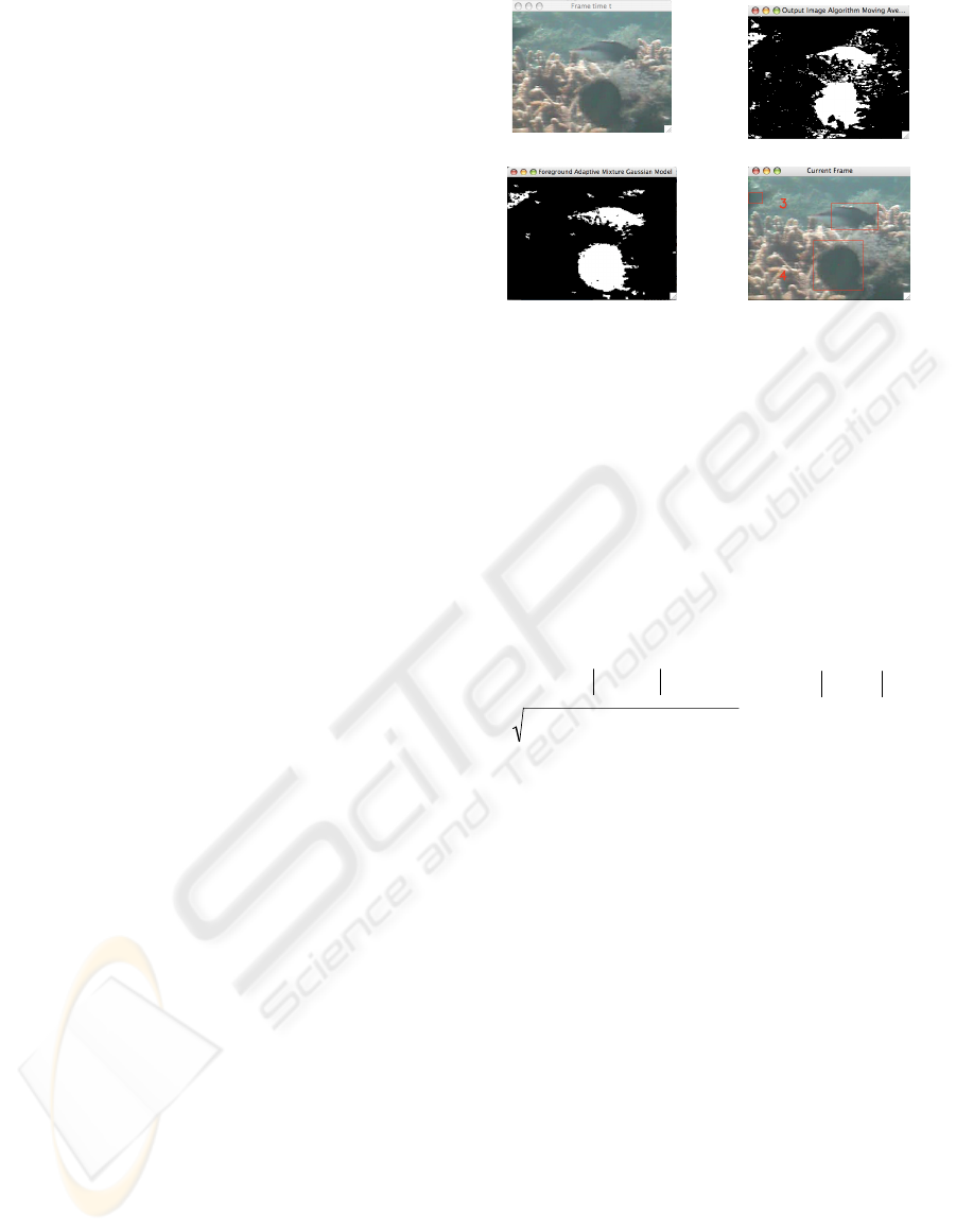
critical parameters, as for example an algorithm

based on Kalman filtering. Alternatively, the

algorithms were too slow.

The algorithm chosen was the Adaptive

Gaussian Mixture Model (Zivkovic, 2004), which

was reliable enough for removing the false positives

and fast enough. In this algorithm, each background

pixel is modeled as a mixture of Gaussians.

Afterwards, each pixel is classified based on the

likelihood that the observed pixel value is explained

by the gaussian mixture model. Figure 3(c) shows

the output of this new algorithm.

If it was used independently, it may fail when

slowly moving objects are present in the scene. The

moving average detection algorithm, on the other

hand, overcomes such problems.

Therefore, a combination of these two

algorithms gave a reliable solution for fish detection,

as each algorithm solves some problems of the other.

Therefore, let AP

be the output image of the

Adaptive Gaussian Mixture Model, therefore the

final output of the proposed algorithm is given by an

“And Operation” between AP

and MP

. To clearly

identify each object in the scene, the “and image” is

further filtered using a morphological filter

combined with size filtering operations. In particular

we have adopted operations of erosions followed by

closing (10 times), dilations followed by opening

(15 times) and median statistic filter (with a kernel

size of 17x17) thus obtaining an output image such

as the one shown in Figure 3(d).

Finally, the number of fish in a frame is now

obtained by applying a connected component-

labelling algorithm. Having detected the fish, it is

now necessary to firstly implement a tracking

algorithm to estimate the total number of individual

fish in a video.

5 TRACKING SYSTEM

We use a combination of two algorithms for

tracking: the first one is based on the matching of

blob shape features and the second one based on the

histogram matching. For the “shape feature

algorithm”, we use

Fis

to denote the i

fish,

detected in frame n. We then use a feature vector

= C

n,x

n,y

n,x

n,y

, A

{}

for representing the

parameters of the i

fish, where

n,x

n,y

(

)

is the

centroid of the fish

Fis

n,x

n,y

(

)

the average

motion vector of the fish

Fis

the area of the

fish

Fis

and

the orientation (in degrees) of the

fish

Fis

(a)

(b)

(c)

(d)

Figure 3: (a) Grabbed Frame, detected foreground by the

(b) Moving Average Detection Algorithm, (c) Adaptive

Gaussian Mixture Model, (d) Final output of the detection

algorithm.

The motion vector is defined as a field of object

velocities at each point in space that defines the 3D

motion of objects in a time varying scene. The

orientation of a blob is defined as the angle

composed by the principal axis of the object and the

vertical axis.

Fis

is compared to the fish in frame

n+1, and

Fis

is matched with

Fis

n +1

if the

following matching rules are satisfied:

− A

n +1

< Th

−

n +1

< Th

n,x

− C

n +1,x

()

+ C

n,y

− C

n +1,y

()

< Th

(8)

Tracking by “colour matching” has been carried

out by applying the Continuously Adaptive Mean

Shift Algorithm (CamShift), which is an adaptation

of the Mean Shift algorithm (Fugunaka, 1990).

Given a probability density image, Camshift

finds the mean (mode) of the distribution by

iterating in the direction of maximum increase in

probability density (Intel Corporation, 2001).

The Probability Distribution Function (PDF) of

images adopted in our work is the Histogram Back-

Projection, which associates the pixel values in the

image with the value of the corresponding histogram

bin. The back-projection of the target histogram with

any consecutive frame generates a probability image

where the value of each pixel characterizes the

probability that the input pixel belongs to the

histogram of the target object. Hence, to generate the

PDF, an initial histogram of the hue channel in HSV

colour space is computed from the initial ROI of the

filtered image. Tracks that are less than 3 frames

long are ignored.

Figure 4 shows example outputs of the tracking

system, where the tracking is illustrated by colouring

the bounding boxes of the detected fish using

DETECTING ,TRACKING AND COUNTING FISH IN LOW QUALITY UNCONSTRAINED UNDERWATER

VIDEOS

517

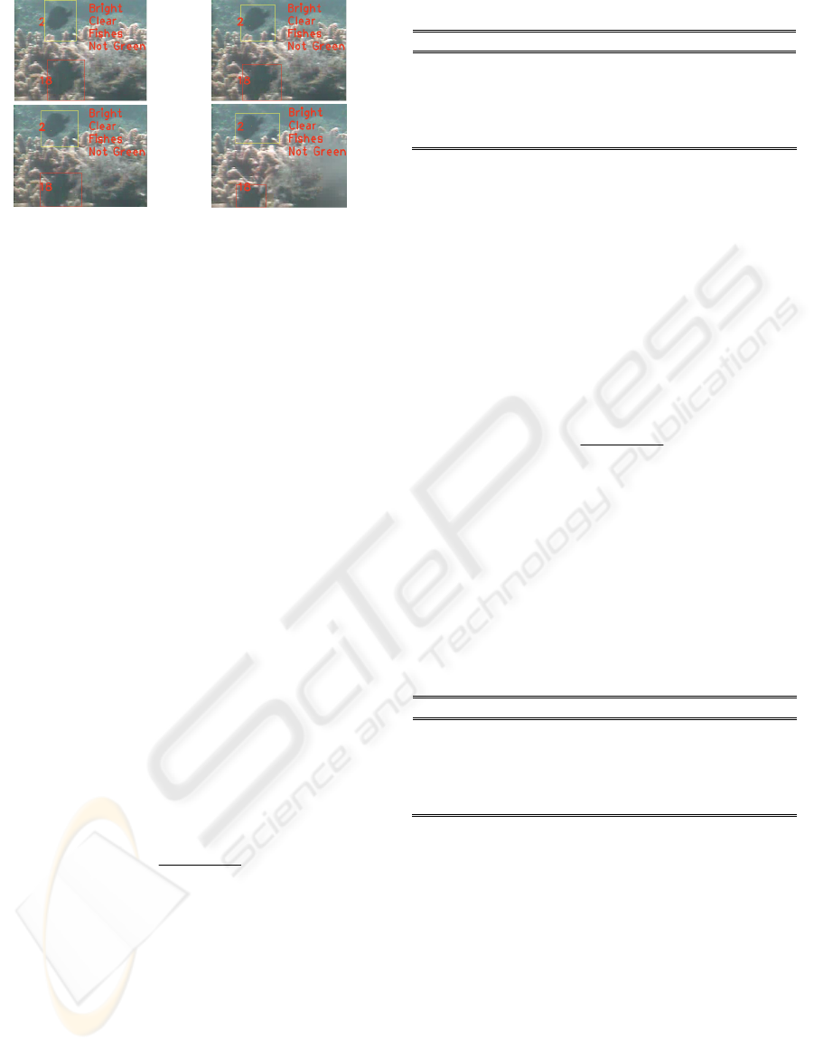
Figure 4: Tracking example with four frames grabbed at

four consecutively times.

different colours (yellow for the one in the upper left

and red for the lower left).

6 EXPERIMENTAL RESULTS

To evaluate the effectiveness of the proposed

system, we tested our method on 20 different

underwater sequences. These video sequences are

sampled to 320×240 with a 24-bit RGB and at a

frame rate of 5fps. Each video is about 1 minute

long (300 frames).

The aim of this experiment is to determine the

accuracy of its fish detection and counting abilities

that make use of the fish tracking modules.

Our system can fail to extract objects of interest,

thus miss out potentially interesting entities. This is

called False Negative (FN). Moreover, it can extract

targets apparently of interest, but in fact, is a false

identification, e.g. by considering a part of

background as foreground. This error is referred to

as False Positive (FP).

We show our experimental results at two

different stages: Fish Detection and Fish Counting.

Table 2 shows the detection results. The

Detection Success Rate (DSR) is defined below:

FPND

DSR

)(

100

−

⋅=

(9)

For each video, NR denotes the real number of

fish in each frame; ND represents the total number

of fish detected using our algorithm; FP and FN,

respectively, store the values of False Positives and

False Negatives. The performance of the detection

algorithm is promising: up to 89.5% and no less than

80% of fish have been correctly detected. The

number of False Positives has occurred due to the

un-controlled open water environment with moving

background objects and videos being shot in murky

waters. This error is largely corrected when the Fish

Tracking algorithm is carried out.

Table 2: Detection Algorithm Results.

Video NR ND FP FN DSR

1 160 146 7 21 86.8%

2 94 80 4 10 80.5%

3 212 198 9 23 89.5%

4 83 74 3 12 85.5%

5 76 65 2 13 81.5%

The Fish Tracking algorithm has shown

excellent results with about 90% accuracy. The 10%

of error was caused by the absence of a sophisticated

fish identification algorithm that would help

distinguish e.g. cases like where two fish pass in

front of each other.

Based on the two previous algorithms, additional

fish counting algorithm is carried out to count the

total number of individual fish in a video. The

overall results for fish counting are given in Table 3.

The Counting Success Rate (CSR) is formulated

below:

OCFC

CSR

)(

100

−

⋅=

(10)

NF is the total number of individual fish in the

entire video. FC is the number of fish counted by the

algorithm. OC is the number of fish overcounted,

due to the failure to detect the same fish in

intermediate frames in the detection algorithm. This

leads the same fish to be tracked several times and

thus overcounted. ND is the number of fish not

detected.

Table 3: Fish Counting Results.

Video NF FC OC ND CSR

1 30 28 1 3 90.0%

2 12 10 0 2 83.3 %

3 54 54 4 4 92.5%

4 12 14 4 2 83.3%

5 12 13 4 3 75.0%

Considering the large amount and different types

of noise that affect these videos, the above findings

of an average success rate of 85.72% over all 20

movies (about 8000 frames) is more than satisfying.

Often the overcounting errors are caused by the low

frame rate presented in the video (fish move too fast

to be successfully tracked) and the low quality of the

images. The obtained results are considered

excellent when compared with other similar

algorithms where fish counting was carried out in a

constrained environment. For instance, (Morais

Erikson et al, 2005) reported a 81% success rate on

fish counting in a constrained environment, i.e. in a

fish tank with fixed number of fish and in a

controlled lab. (Petrell et. al.,1997) and (Ruff et. al.

1995) proposed video-based systems to measure fish

VISAPP 2008 - International Conference on Computer Vision Theory and Applications

518

number and average fish size with images taken in

bordered cages.

The algorithm, implemented in C++ with Intel

OpenCV 1.0 library, takes about on average 85

seconds for processing a video of 60 seconds on a

Intel Core 2 Duo 2.0GHz with a 1GB Ram. The

same system operates close to real time performance

using an Intel Core 2 Duo Extreme 2.8GHz.

7 CONCLUSIONS AND FUTURE

WORK

This paper presented a machine vision system that

automatically determines and annotates

characteristics of underwater video images. The

main goal of our system is to provide marine

biologists with useful analysis therefore allowing

them to cut down viewing and searching time of raw

videos. Examples of analysis done are the

identification of environmental conditions (e.g. the

brightness or smoothness of a video), the numbers of

fish present in a frame (therefore helping locate

useful frames in a video), the total number of fish in

a video (help selecting between videos) and the

overall quality of a video (helping select videos

based on desirable qualities). We note that the

observed accuracy of 85% may be considered as a

satisfactory estimate, since it provides a reasonable

approximation of the actual fish flow, the varying

environmental conditions in an open unconstrained

space and the changeable status of the sensors used.

Unlike other existing fish image processing

methods which are mostly conducted in a lab, our

approach provides a reliable method where analysis

are carried out on data captured in their natural

habitat where conditions may vary drastically which

inevitable introduced uncontrollable interferences,

e.g. murky water, algae on camera lens, moving

plants and unknown objects, low contrast, low frame

rates, etc.

Further development for fish classification and

occlusion handling is in progress. Fish classification

for the EcoGrid videos is a very challenging task due

to the low quality images and varying scenarios that

need to be taken into account.

New algorithms for detection and tracking will

be implemented in order to investigate improved

efficiency. Furthermore, the algorithms developed to

perform the video analysis, (such as pre-processing,

detection, tracking and counting) could be integrated

into a more generic architecture so that the best

algorithm for each step will be selected. The

performance level for the algorithms will be

determined by a measure such as processing time or

certain user provided requirements. Thus a

combination of optimal algorithms to perform the

video analysis could be utilized.

REFERENCES

Brehmera, P., Do Chib, T., Mouillotb D., (2006)

Amphidromous fish school migration revealed by

combining fixed sonar monitoring (horizontal

beaming) with fishing data. Journal of Experimental

Marine Biology and Ecology. Vol. 334, Issue 1, pp.

139-150.

Petrell, R. J, Shi X, Ward R. K., Naiberg, A. and Savage

C. R. (1997) Determining fish size and swimming

speed in cages and tanks using simple video

techniques, Aquacultural Engineering, Vol.16, pp. 63-

84.

Faro A., Giordano D., Spampinato C. (2004). Soft-

Computing Agents Processing Web Cam Images To

Optimize Metropolitan Traffic Systems, LNCS, Book

CVG, Netherlands, Vol. 32, pp. 968-974.

Fugunaga, K. (1990): Introduction to Statistical Pattern

Recognition, 2nd Edition, Academic Press, NY, 1990.

Intel Corporation (2001): Open Source Computer Vision

Library Reference Manual.

Morais Erikson F., Campos Mario F. M., Pádua Flávio L.

C. and Carceroni Rodrigo L. (2005) “Particle Filter-

based Predictive Tracking for Robust Fish Counting”,

2005 SIBGRAPI, pp: 367 - 374

Otsu N. (1979) “A Threshold Selection Method from

Gray-Level Histograms”, IEEE Transactions on SMC,

vol. 9, pp. 62-66.

Rajagopalan N., Burlina P., Chellappa P. (1999) “Higher

Order Statistical Learning for Vehicle Detection in

Images”, Proceedings of ICCV99, 20-25 September,

Corfu, Greece.

Ruff, B. P., Marchant J. A., and Frost A. R. (1995) “Fish

sizing and monitoring using a stereo image analysis

syste applied to fish farming”. Aquacultural

Engineering, Vol. 14, pp.155-173.

Rouse W. (2007). Marine Biology Research Experiment:

Population Dynamics of Barnacles in the Intertidal

Zone. May 27, 2007.

Schlieper, C. (1972). Research methods in marine biology.

University of Washington Press, Seattle, 1972.

Zivkovic Z. (2004) Improved adaptive Gausian mixture

model for background subtraction, Proceedings of

ICPR 2004, August 23-26, Cambridge, UK.

DETECTING ,TRACKING AND COUNTING FISH IN LOW QUALITY UNCONSTRAINED UNDERWATER

VIDEOS

519