CONSTRAIN PROPAGATION FOR GHOST REMOVAL IN HIGH

DYNAMIC RANGE IMAGES

Matteo Pedone and Janne Heikkilä

Machine Vision Group, Department of Electrical and Information Engineering, University of Oulu, Finland

Keywords:

Motion detection, density estimation, image fusion, energy minimization.

Abstract:

Creating high dynamic range images of non-static scenes is a challenging task. Carefully preventing strong

camera shakes during shooting and performing image-registration before combining the exposures cannot

ensure that the resulting HDR image is consistent. This is eventually due to the presence of moving objects

in the scene that causes the so called ghosting artifacts. Currently there is no robust solution that produces

satisfactory results in any circumstance. Our method consists of two main steps. First, the probability of

belonging to the static part of the scene is estimated for each pixel of the N exposures, yielding N weight

images. In the second phase, we segment the areas of the weight-images with lower and higher probability

values, and smoothly propagate their inﬂuence until a signiﬁcant change in luminosity is detected or a pixel

with a corresponding high probability of belonging to the background is approached. This represents an

attempt to spread the inﬂuence of lower weights to the surrounding pixels of the same object. Results produced

with our technique show a signiﬁcant reduction or total removal of ghosting artifacts.

1 INTRODUCTION

High dynamic range images are commonly created by

combining a set of images acquired with varying ex-

posure time (Debevec and Malik, 1997). Ideally, the

information contained in the pixels of one exposure

must be combined with the corresponding pixels of

the other exposures representing the same features of

the scene. This is usually accomplished by attempting

to avoid camera shakes during shooting and by per-

forming an extra image registration step before merg-

ing the exposures. However, although this may maxi-

mize the overlap between the exposures, it is not pos-

sible to guarantee that the same spatial locations in

the low dynamic range images represent the same de-

tails of the scene; this is due to the non-static nature

of most scenes encountered in practical applications.

This situation eventually occurs in the regions of the

image space where movement was present or where

the image registration algorithm failed to properly

align the shots. Combining an exposure set suffering

from such inconsistencies will surely cause ghosting

artifacts to be visible in the resulting HDR image, in

the form of semi-transparent features. Unless ghost-

ing is involved only in a reasonably small area of the

image, it usually produces unacceptable results; this

restricts the use of high dynamic range imaging only

to static scenes.

2 PREVIOUS WORK

Some authors treat ghosting as an analogous prob-

lem to image-registration; a possible solution would

then be tracking object movements across the expo-

sures and use this information to warp the pixels of

the images accordingly, in order to produce an ac-

curate alignment (Bogoni, 2000). These techniques

rely on motion estimation by optical-ﬂow, and it is not

possible to ensure they work properly with any kind

of movement; for example they inevitably fail when

details in some exposures do not have any correspon-

dence in others, due to occlusion.

Ward in (Reinhard et al., 2005) proposes to de-

tect and segment movement regions and replace each

segment with information extracted from a single ex-

Pedone M. and Heikkilä J. (2008).

CONSTRAIN PROPAGATION FOR GHOST REMOVAL IN HIGH DYNAMIC RANGE IMAGES.

In Proceedings of the Third International Conference on Computer Vision Theory and Applications, pages 36-41

DOI: 10.5220/0001076300360041

 SciTePress

posure. Movement is detected using a measure based

on a weighted variance of pixel values across the ex-

posures, for each location; regions are then selected

by marking only the locations where the variance ex-

ceeds a threshold value. The main drawback of this

method is that ghost regions are replaced by pixels

from a single reference image; if a segmented ghost

occurs in an area where the dynamic range is high,

any exposure will contain underexposed or saturated

pixels in that area (or eventually both). Moreover the

weighted variance, does not always work properly as

a measure for detecting movement; in particular it

usually fails when the pixel values of the moving ob-

ject are similar to those of the background. This moti-

vated Jacobs et al. in (Jacobs et al., 2005) to introduce

an auxiliary measure based on entropy that is insen-

sitive to the amount of contrast in the pixel data and

efﬁciently allows to detect movement of features that

are similar to the background; nonetheless detected

areas are again replaced with pixels of a single expo-

sure.

Grosch in (Grosch, 2006) describes a similar ap-

proach based on the idea that the functions that map

the intensity of any pixel of one exposure to the cor-

responding intensity in another exposure can be re-

trieved, if the camera response function and the expo-

sure times are known. He then uses such functions to

predict pixel values across the exposures and create

an error map. The error map is thresholded in order

to mark invalid locations, that are replaced with pixels

from one or possibly more exposures. The algorithm

however cannot remove ghosts whose colors are sim-

ilar to the ones of the background, and the dynamic

range in movement areas remains limited.

A different approach is described in (Khan et al.,

2006) and it consists in assigning to each pixel of ev-

ery exposure its probability of belonging to the back-

ground. The weights used for pixel values when com-

bining the exposures, are then chosen to reduce the

effect of underexposed or saturated pixels as well as

to reduce the inﬂuence of pixels with a low likeli-

hood of belonging to the background. The procedure

used in order to compute these probabilities can be

eventually reiterated to get progressively more accu-

rate results. The method, although computationally

expensive compared to the others, works fairly well

as long as the exposures prevalently capture the back-

ground, and it is able to reduce ghosting artifacts in

regions where the dynamic range is high. However

the algorithm is based on non-parametric kernel den-

sity estimation whose efﬁciency is dependent on a

good choice of the smoothing parameters. In addition

a density estimation approach is applied to data sets

that are not suitable, since analogous elements even-

tually correspond to different values due to variations

in overall brightness across the exposures.

3 DETECTING BACKGROUND

PIXELS

We treat ghosting as an analogue problem of detect-

ing pixels belonging to the static part of the scene (the

background). First, for each location in image space,

a statistical model of the background is created, based

on information related to the pixels of a neighbor-

hood; successively, the chance of belonging to this

class is evaluated for the pixels of interest. A low

probability is likely to be a caused by the local pres-

ence of ghosts. Our approach shares similarities with

the iterative scheme suggested in (Khan et al., 2006),

however we bring important improvements that make

it more suitable for high dynamic range applications

and lead to a superior removal of ghosts, as shown in

our results.

A three-element vector of the form (c

, c

) ∈

ℜ

is associated to an arbitrary pixel; its elements cor-

respond to the color information of that pixel. Let

R be the total number of exposures; for each spa-

tial location (i, j) the set N

i, j

of neighboring pixels

is used as an approximate representation of the back-

ground and it is deﬁned as N

i, j

= { f (x, y, r) | r ∈

[1..R], i−1 ≤ x ≤ i+1, j −1 ≤ y ≤ j +1, x 6= i, y 6= j},

where f (x, y, r) ∈ ℜ

denotes the three-components

pixel color values at coordinates (x, y) in the r-th ex-

posure. If we think of an exposures sequence as a

M × N × R image, N

i, j

can be seen as the set of all the

pixels in a rectangular 3 × 3 × R region in 3d-space

excluding all the central pixels. The probability p for

a pixel at coordinates (i, j, r) with r = 1..R of belong-

ing to the class N

i, j

is estimated by a non-parametric

kernel density estimation approach. The probabilities

p(x) where x ∈ ℜ

denotes a generic pixel vector, are

then given by

ˆp(x) =k H k

−1

∑

i=1

w(X

)K(H

−1

(x −X

))

∑

i=1

w(X

)

. (1)

N is the total number of samples, the vectors X

are

the sample pixels that constitute the model of the

background, w is a weight function that limits the in-

ﬂuence of those pixels that are under-exposed or sat-

urated, and have little chance to be part of the back-

ground; the latter is achieved by reusing the values

ˆp(

x) from the previous iteration of the algorithm as

described in (Khan et al., 2006). K is a d-variate ker-

nel function, and H is a symmetric positive deﬁnite

d × d bandwidth matrix.

CONSTRAIN PROPAGATION FOR GHOST REMOVAL IN HIGH DYNAMIC RANGE IMAGES

Since the particular shape of the kernel function

generally does not have a critical impact in perfor-

mance terms (Silverman, 1986), a standard multivari-

ate Gaussian kernel with identity covariance matrix is

often a reasonable choice for K, that is

K(x) =

(2π)

exp(−

x) (2)

On the other hand it is well known that the use of

density estimation approaches can bring useful results

only when the bandwidth values (or alternatively,

smoothing parameters) are properly set. Non-suitable

bandwidth values are the cause of undersmoothing or

oversmoothing (Silverman, 1986), and for this reason

their importance is to be considered vital. Moreover,

the “goodness” of the smoothing parameters strongly

depends on the nature of the data set in question that

could signiﬁcantly change between different locations

in image space. In addition, it must be mentioned that

density estimation approaches work correctly as far as

same observations correspond to equal vector values

in the data set of samples, and this is not the case for

high dynamic range applications, due to overall inten-

sity variations across the exposures.

3.1 Pre-Transforming Pixel Values

Density estimation is a reasonable approach as long

as analogue observations of a quantity actually corre-

spond to equal sampled values. However the variation

in pixel intensity between any pair of exposures can

be described by an intensity-mapping-function (IMF)

i, j

that maps the brightness of an arbitrary pixel in

the i-th exposure into the corresponding brightness

in the j-th exposure. Often, only the subset of IMFs

between adjacent exposures is considered, where

stands for τ

i,i+1

. It has been proved that IMFs

are theoretically always monotonic increasing (Gross-

berg and Nayar, 2003). Let’s have a sequence of R

exposures and let c be a pixel value; the functions

(r) = τ

r−1

(...(τ

(c))), where r ∈ [1, R] and τ

c, describe how the intensity of corresponding pixels

varies in function of the exposure number. A function

, given by the composition of monotonic increas-

ing functions, is monotonic increasing too; from this

it follows it has an inverse. However IMFs in prac-

tice do not describe the accurate correspondence be-

tween pixel intensities due to factors such as clamp-

ing, quantization errors and noise, that usually have a

signiﬁcant inﬂuence in darker and brighter areas of an

image. This suggests the introduction of a valid pixel

range, typically V = [20, 240], where the mentioned

factors can be considered negligible to some extent.

Considering only pixel values c ∈ V , and an arbitrary

exposure s, the function

(r; s) =



r−1

(...(τ

(c))) r > s

c r = s

can be considered monotonic increasing in the inter-

val s ≤ r ≤ l, where l = max{r |

(r; s) ∈ V }. This

intuitively suggests that intensities of corresponding

well exposed pixels can and should be transformed

into the same value.

We only experimented with a naive approach

based on histogram matching. We choose the “best”

reference exposure of the sequence and perform a “re-

laxed” intensity alignment to it for all the other expo-

sures. We typically choose the exposure whose in-

tegral of the luminance channel histogram in the in-

tervals [0, 20] and [240, 255] is lowest, preferring the

one that uses more bins. Intensity alignment is per-

formed by simple histogram matching, although for

this application a more robust radiometric alignment

approach like the one described in (Kim and Polle-

feys, 2004) could be eventually used. We reduce

the loss of information due to intensity alignment, by

introducing a simple measure of its “harmfulness”.

Let’s have two images A, B and denote by A → B the

resulting image of an intensity-alignment of A to B (A

matches B). We attempt to quantify the loss of infor-

mation due to the intensity-alignment operation by

loss

A,B

| {hist

((A → B) → A) > 0} |

| {hist

(A) > 0} |

where hist

(X) is the luminance channel histogram

of an image X, and | {hist

(X) > 0} | returns the to-

tal number of used bins. This is justiﬁed by the fact

that transforming an image A into A → B would most

likely cause a certain amount of pixels to be clamped

to the valid color range, and transforming A → B back

to its original intensity would yield a resulting image

(A → B) → A suffering from posterization artifacts.

The quantity loss

A,B

is in the range (0, 1] and it is

used to deﬁne a linear interpolation factor t between

the original image and the intensity-matched version

of it, in the following way,

t =



k k ≤ 1

1 k > 1

where

k =

loss

A,B

1−tolerance

0 ≤ tolerance < 1

and the factor tolerance determines when to start to

linearly interpolate. We set by default tolerance =

0.3. Density estimation is ﬁnally performed on the

set of intensity-aligned images (with opportune “re-

laxation”), while the output weights of the algorithm

are of course used with the original set of exposures.

VISAPP 2008 - International Conference on Computer Vision Theory and Applications

3.2 Estimating Bandwidth Matrices

In (Raykar and Duraiswami, 2006) Vikas et al. de-

scribe methods to quickly compute the optimal band-

width value for univariate data, and in (Zhang et al.,

2004) an algorithm to estimate full bandwidth matri-

ces in the multivariate case is proposed. A natural ap-

proach would then be applying such algorithms to the

pixel data contained in N

i, j

, and repeating this step at

each location (i, j); nevertheless the amount of calcu-

lations required would become unacceptable. Using a

decorrelated color space like Lαβ or CIELAB makes

the choice of a product kernel (H diagonal) reason-

able. This led us to consider the possibility of estimat-

ing the bandwidth parameters using a straightforward

and fast method. We used a slightly modiﬁed version

of Scott’s rule (Scott, 1992), that in its original form

≈ n

−

d+4

where d is the dimensionality of the n samples, and σ

is their standard deviation in the i-th dimension. Con-

cerning the terms σ

, we prefer to compute weighted

standard deviations of the following form,

σ =

∑

i=1

w(x

) ·(x

− ˜x)

∑

i=1

w(x

)

where w(x

) are the sample weights, ˜x is the weighted

mean of the samples x

, and n is the total number of

samples. We use the pixel weights obtained from the

last iteration of the algorithm to reduce the inﬂuence

of the pixels that are incorrectly exposed and have lit-

tle chance of belonging to the background. We ﬁnally

propose the following bandwidth matrix for an arbi-

trary neighborhood set N

i, j

i,j



i, j



−

diag



i, j

)



(3)

where we respectively denoted by

i, j

)

and

i, j

) the weighted standard deviations of the

luminance and color data of the pixels of the neigh-

borhood N

i, j

In addition, it is possible to obtain satisfactory re-

sults and save computation time by precalculating the

set of matrices H

i,j

in the beginning and reusing it at

every iteration, or alternatively by applying (3) to the

entire set of pixels of all the exposures in order to ob-

tain only one global suitable bandwidth matrix.

3.3 Weights Propagation

It often happens that although some portions of a

moving object are correctly detected and assigned

low probabilities of belonging to the static part of the

scene, other parts are still given higher weights. This

can be due to several reasons like similarity of object

and background colors, or more generally to limita-

tions in the density estimation approach. Intuitively,

if a portion of a moving object has low chances of

belonging to the background, this should be eventu-

ally valid also for all the other portions of the same

object. We describe a method that attempts to prop-

agate the inﬂuence of the lower probabilities to the

surrounding areas of the image representing the same

feature. After each iteration of the procedure de-

scribed in the previous sections, a new M ×N ×R ma-

trix of normalized weights is available. Before merg-

ing the exposures, we compute two threshold values

to segment the areas with relatively low and high like-

lihood of being part of the static part of the scene;

the values we use are respectively the 10-th percentile

and the 60-th percentile of all the pixel weights. For

each exposure, two morphological operation are ap-

plied to the binary images relative to the lower and

higher weights: respectively close and open using a

disc shaped structuring element of 7 pixels radius.

The former image is multiplied by a low value (we

use 0.01), and its nonzero pixels replace the corre-

sponding ones in the latter image. This procedure

yields R constrain-images that can be used in conjunc-

tion with the original exposures to perform an image-

driven propagation; the approach used is the one de-

scribed in (Lischinski et al., 2006) that minimizes the

following quadratic functional:

f = arg min



∑

w(x)( f (x) − g(x))

+λ

∑

(x)

+ ε



(x)



(x)



+ ε

Intuitively the ﬁrst term aims to keep the resulting

pixel weights given by f, as close as possible to the

values g(x) of the constrain-image, while the second

term is necessary to keep the gradient of the objec-

tive function small, allowing however large changes

when the gradient of the log-luminance channel L of

the underlying image is signiﬁcant. The weights w(x)

and the parameters λ, α, and ε can be used to control

the type of propagation; in our experiments we used

the default values λ = 0.2, α = 1, ε = 0.0001, while

w(x) is equal to 1 in correspondence of the nonzero

values of the constrain image, and 0 otherwise. The

propagated weights are then multiplied element by el-

ement by the original weight matrix, and used either

to combine the exposures, or to perform an extra it-

eration of the algorithm (Figure 1). Lischinski et al.

in their paper describe a fast method that is able to

minimize the functional f in a fraction of second for a

640 × 400 image. In order to save memory and com-

CONSTRAIN PROPAGATION FOR GHOST REMOVAL IN HIGH DYNAMIC RANGE IMAGES

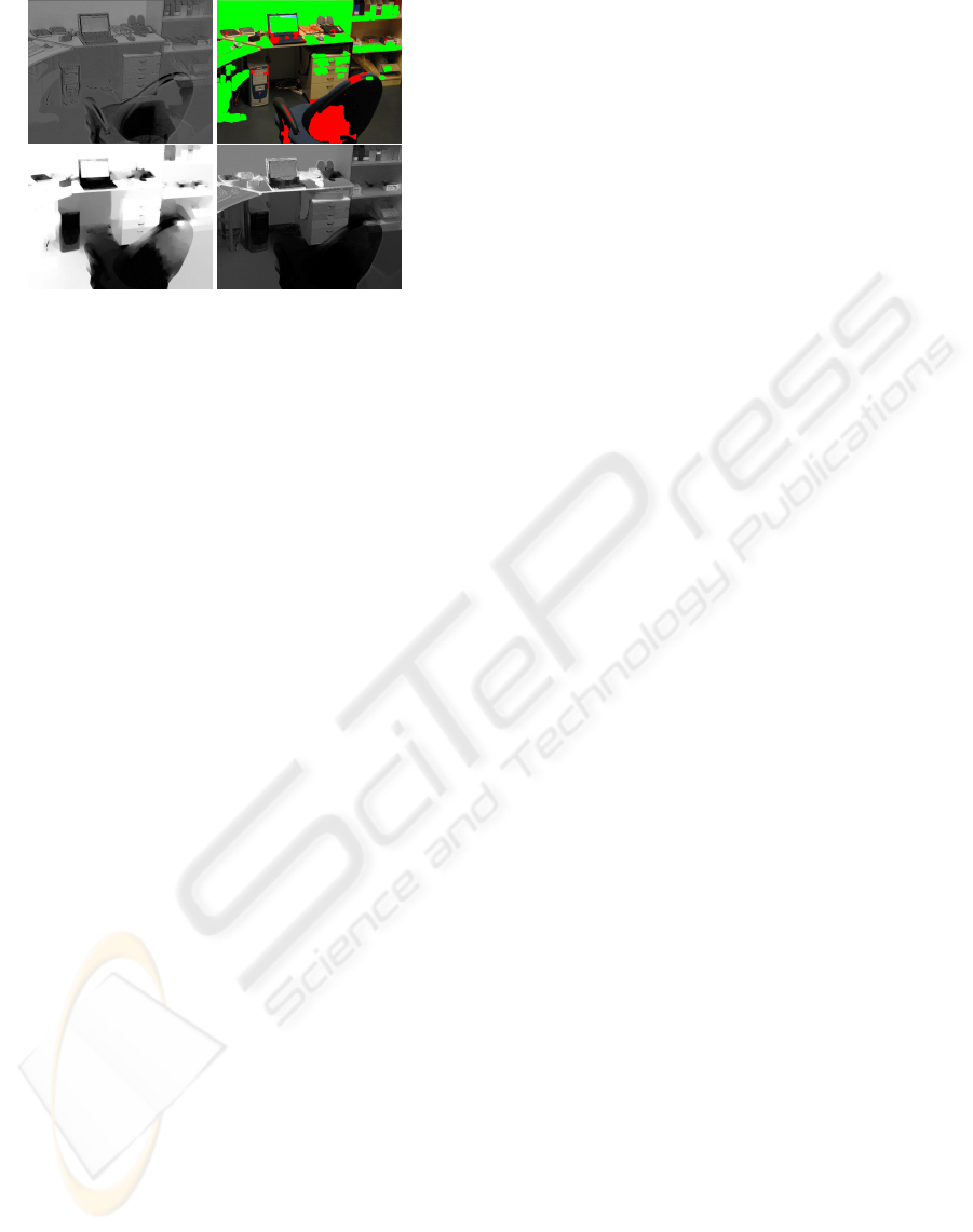
Figure 1: The main steps of the propagation process:

weights obtained from density estimation; low and high

weights segmented; propagated weights; ﬁnal weights.

putation time, in case of big images, we perform the

propagation step on downsampled versions of the ex-

posures, and resize the results back to their original

dimensions.

4 RESULTS AND CONCLUSION

We compared our approach to the one described in

(Khan et al., 2006). Reinhard’s photographic opera-

tor was used to tonemap the generated HDR images

(Reinhard et al., 2002). Our approach does not require

any setting to be adjusted by the user. In all the exper-

iments shown we used only one global bandwidth ma-

trix that is reused at every iteration: the more general

approach described resulted in a signiﬁcant increase

of computation time with little beneﬁts. For Khan’s

method, we used a default identity bandwidth matrix,

and 3 × 3 × R neighborhoods. We included in Figure

2 some of the exposures used for generating the ﬁnal

HDR images. Figure 3 shows the results of the exper-

iments. In the ﬁrst scene, ghosting is localized and oc-

curs in regions that have high dynamic range; artifacts

are completely removed only with our algorithm. In

the second scene, the situation is similar but less expo-

sures were available. Density estimation alone could

not distinguish properly the background, while the

weight propagation helped to improve the results. Fi-

nally we considered a handheld set of exposures in-

tentionally left unaligned, and where chaotic move-

ment is present; this sequence does not hold the as-

sumption that the background is prevalently captured

and suffers from critical occlusion and parallax prob-

lems. In spite of this, our method proved a remarkable

robustness against feature misalignments. In all the

cases that have been considered, our approach showed

a signiﬁcant improvement in reducing ghosting arti-

facts, and when the previously mentioned assumption

holds, ghosts can be completely eliminated even with

a single iteration.

REFERENCES

Bogoni, L. (2000). Extending dynamic range of

monochrome and color images through fusion. In In-

ternational Conference on Pattern Recognition, 2000,

vol. 3, pp. 7-12.

Debevec, P. and Malik, J. (1997). Recovering high dynamic

range radiance maps from photograph. In SIGGRAPH

97, August 1997.

Grosch, T. (2006). Fast and robust high dynamic range

image generation with camera and object movement.

In Vision, Modeling and Visualization (VMV), RWTH

Aachen, 22.11 - 24.11.2006.

Grossberg, M. D. and Nayar, S. K. (2003). Determining the

camera response from images: What is knowable? In

IEEE Transactions on Pattern Analysis and Machine

Intelligence, Vol.25, No.11, pp.1455-1467, Nov, 2003.

Jacobs, K., Ward, G., and Loscos, C. (2005). Automatic

hdri generation of dynamic environments. In ACM

SIGGRAPH 2005 Sketches.

Khan, E. A., Akyuz, A. O., and Reinhard, E. (2006). Ghost

removal in high dynamic range images. In IEEE In-

ternational Conference on Image Processing, Atlanta,

USA, August 2006.

Kim, S. J. and Pollefeys, M. (2004). Radiometric alignment

of image sequences. In IEEE Computer Society Con-

ference on Computer Vision and Pattern Recognition

(CVPR’04) - Volume 1, pp. 645-651.

Lischinski, D., Farbman, Z., Uyttendaele, M., and Szeliski,

R. (2006). Interactive local adjustment of tonal val-

ues. In ACM Transactions on Graphics, ACM SIG-

GRAPH 2006 Papers SIGGRAPH ’06, Volume 25 Is-

sue 3. ACM Press.

Raykar, V. C. and Duraiswami, R. (2006). Very fast opti-

mal bandwidth selection for univariate kernel density

estimation. In CS-TR-4774, Department of Computer

Science, University of Maryland, Collegepark.

Reinhard, E., Stark, M., Shirley, P., and Ferwerda, J. (2002).

Photographic tone reproduction for digital images. In

ACM Transactions on Graphics, 21(3), pp 267-276,

Proceedings of SIGGRAPH 2002.

Reinhard, E., Ward, G., Pattanaik, S., and Debevec, P.

(2005). High Dynamic Range Imaging: Acquisition,

Display and Image-Based-Lighting. Morgan Kauf-

mann.

Scott, D. W. (1992). Multivariate Density Estimation: The-

ory, Practice, and Visualization. John Wiley.

Silverman, B. W. (1986). Density Estimation for Statistics

and Data Analysis. Chapman and Hall.

Zhang, X., King, M. L., and Hyndman, R. J. (2004). Band-

width selection for multivariate kernel density estima-

tion using mcmc. In Monash Econometrics and Busi-

ness Statistics Working Papers 9/04.

VISAPP 2008 - International Conference on Computer Vision Theory and Applications

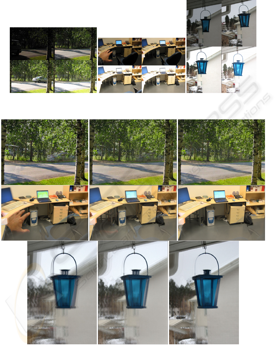
Figure 2: Some of the exposures used in the experiments. From left to right, the original sequences contained respectively

seven, ﬁve, and six exposures.

Figure 3: Results obtained without any ghost removal applied (left column); with Khan’s method (middle column); with our

method (right column). Six iterations of Khan’s method have been used for the ﬁrst two sequences, and four iterations for the

third one; further iterations did not improve signiﬁcantly the ﬁnal image. All the results produced with our method required

only a single iteration. In the ﬁrst sequence, ghosting artifacts of the car on the right are completely removed only with our

algorithm. The propagation approach works fairly well also with ghosting artifacts caused by feature misalignments.

CONSTRAIN PROPAGATION FOR GHOST REMOVAL IN HIGH DYNAMIC RANGE IMAGES