USING
LOW-LEVEL MOTION TO ESTIMATE GAIT PHASE
Ben Daubney, David Gibson and Neill Campbell
Department of Computer Science, University of Bristol, Bristol, BS8 1UB, UK
Keywords:
Dynamic Programming, Gait Phase Estimation, Human Tracking.
Abstract:
This paper presents a method that is capable of robustly estimating gait phase of a human walking using the
motion of a sparse cloud of feature points extracted using a standard feature tracker. We first learn statistical
motion models of the trajectories we would expect to observe for each of the main limbs. By comparing the
motion of the tracked features to our models and integrating over all features we create a state probability
matrix that represents the likelihood of being at a particular phase as a function of time. By using dynamic
programming and allowing only likely phase transitions to occur between consecutive frames, an optimal
solution can be found that estimates the gait phase for each frame. This work demonstrates that despite the
sparsity and noise contained in the tracking data, the information encapsulated in the motion of these points is
sufficient to extract gait phase to a high level of accuracy. Presented results demonstrate our system is robust
to changes in height of the walker, gait frequency and individual gait characteristics.
1 INTRODUCTION
There is currently much interest in developing sys-
tems that are capable of extracting human body pose
from video sequences. Applications for such a system
include motion capture, medical analysis and surveil-
lance. The emergence of gait as a biometric has par-
ticulary increased interest in being able to recognise
and identify gaited motions. The difficulty in this
problem is that the human body has many degrees of
freedom, each limb alone is capable of a large range
of movements. The result of this is a very compu-
tationally large search space that is inherently multi
modal. Accurately estimating gait phase could be
used to constrain this problem given that at each phase
certain poses are more likely than others.
Particle filters have been used to successfully search
this high dimensional space (Sidenbladh et al., 2000;
Deutscher et al., 2000). This approach does not guar-
antee to find the global minimum and the number of
particles needed grows exponentially with the num-
ber of dimensions being searched. Attempts to over-
come these problems have included the use of an-
nealing (Deutscher et al., 2000) and the use of prior
models that can be used to guide particles to explore
only likely human poses (Caillette et al., 2005). Tech-
niques such as PCA have also been used to reduce
the dimensionality of the problem, thus significantly
reducing the size of the search space (Hu and Bux-
ton, 2005; Urtasun et al., 2005; Argawal and Triggs,
2004).
An image sequence contains a temporal dimension
that can be exploited with the use of a motion model.
Motion models currently used in the literature vary in
how much prior knowledge they encapsulate and sub-
sequently how much they constrain the search space.
Motion models used to track the upper body include
the use of HMMs to ensure smooth trajectory through
a feature space (Navaratnam et al., 2005) and sim-
ple dynamical models to limit the movement of a part
between consecutive frames (Micilotta et al., 2006).
These approaches do not constrain the types of mo-
tion that can be observed, they are not action spe-
cific. Whilst their generality make them attractive
they do not offer enough constraint to yield good re-
sults whilst tracking the entire human body due to self
occlusions and view point ambiguities.
When extracting pose for the entire body it is often
necessary to learn a different motion model for each
action being performed. Often these motion mod-
els can be represented as a curve through a feature
space such as those discussed above. Different po-
sitions on this motion curve can be seen to represent
different phases of a gait cycle and define the expected
pose for each phase. Navigation through this feature
space has been achieved using Extended Kalman Fil-
ters (Hu and Buxton, 2005), Particle Filters (Siden-
bladh et al., 2000) and HMMs (Caillette et al., 2005;
496
Daubney B., Gibson D. and Campbell N. (2008).
USING LOW-LEVEL MOTION TO ESTIMATE GAIT PHASE.
In Proceedings of the Third International Conference on Computer Vision Theory and Applications, pages 496-501
DOI: 10.5220/0001073604960501
Copyright
c
 SciTePress

Lan and Huttenlocher, 2004). These all represent ex-
amples of high-level motion models, since the motion
represents a change in configuration rather than the
movement of individual parts.
The motion of tracked feature points has been used in
the analysis and recognition of quadruped gait (Gib-
son et al., 2003). In this approach tracking errors are
overcome by first splitting the foreground object into
quadrants and then analysing the average motion of
each quadrant. This approach relies on being able to
accurately locate the centre of the foreground object
making it sensitive to outliers.
Gait has successfully been detected using approaches
such as spatio-temporal features (Schuldt et al.,
2004), symmetry cues (Havasi et al., 2007) and prob-
abilistic models learnt from sparse motion features
(Song et al., 2001). However, these approaches do
not estimate the particular phase of gait only that it is
present.
In this work we present a system that exploits the
low-level motion of a sparse set of feature points ex-
tracted using the Kanade-Lucas-Tomasi (KLT) fea-
ture tracker (Shi and Tomasi, 1994). The feature
points track both the foreground and background of
the image meaning segmentation must be carried out.
The feature points also contain tracking errors that are
not gaussian in nature but systematic due to for exam-
ple edge effects, this is particularly apparent during
self occlusion e.g. as one leg passes another.
We initially learn motion models that represents the
expected trajectories for each of the main limbs.
Given a set of feature points we use our models to
simultaneously solve two problems: the first problem
is that of labelling the feature points as belonging to
the background or foreground, if a feature is classified
as a foreground point it is also assigned to the limb
that the feature’s motion best represents. The second
problem is to estimate the phase that the limb must be
in to have produced the observed motion.
Once all feature points have been classified we then
integrate over all the points and estimate the most
likely gait phase for each frame, ensuring that only
smooth transitions are allowed between frames. This
is achieved without making assumptions about the lo-
cation of any of the features; each trajectory is classi-
fied depending only on its motion, not its position.
2 LEARNING
Our objective is to learn a statistical model for each
of the main limbs that represents how we would ex-
pect a point located at that limb to move through time.
To create a motion model we use a representation
similar to (Coughlan et al., 2000) except we make
our representation dependant on orientation; we as-
sume that people walk upright. A different motion
model is learnt for each limb and is represented as
a chain of m vectors, where each vector represents
the mean displacement you would expect to observe
between frames. Each vector also defines the cen-
tre of a Gaussian that represents the variation in mo-
tion we expect. This model can be defined by the
parameters Θ = (R, Σ), where R = {R
1
, .., R
m
} and
Σ = {Σ
1
, .., Σ
m
}. R
j
is the average motion belong-
ing to the jth point in the chain and Σ
j
is the cor-
responding covariance matrix. This representation is
illustrated in Figure 1.
1
∑
),(R
111
θ r
),(R
222
θ r
),(R
333
θ r
),(R
444
θ r
2
∑
3
∑
4
∑
Figure 1: Chain used to represent a motion trajectory. r is
the magnitude of the vector; θ is the angle relative to the
horizontal; Σ is the covariance matrix.
To learn a model for each limb consider we have
a set of example gait cycles {g
1
, .., g
n
} where each
gait cycle consists of m temporally ordered vectors
{
v
1
, ..,
v
m
}
. We want to learn a model
Θ
max
that max-
imises
P(g
1
, .., g
n
|Θ) =
n
∏
i=1
m
∏
j=1
p(g
i
j
|Θ
j
) (1)
This is a maximisation over all the training examples
for every position in the model. We see that equation
(1) can be maximised by solving for each Θ
j
indepen-
dently,
Θ
max
j
= arg max
Θ
j
n
∏
i=1
p(g
i
j
|Θ
j
) (2)
This is the Maximum Likelihood estimate for Θ
j
and
can be calculated directly from the training examples.
Each position j in the model can be seen as represent-
ing a different gait phase.
However, our ground truth data consists of coarsely
hand labeled x and y positions of the main limbs
through the duration of a video clip. To use the
method described above we need examples of indi-
vidual gait cycles and we need all gait cycles to have
the same temporal length.
The data can be cut into individual gait cycles by us-
ing a reliable heuristic, for example the turning point
in the data that corresponds to when the toes are at
their maximum height. To make each gait cycle the
same temporal length the average length is first calcu-
lated. A Cubic spline is then fitted to each individual
USING LOW-LEVEL MOTION TO ESTIMATE GAIT PHASE
497

gait cycle and each gait cycle is resampled to be the
same length as the mean.
These statistical models allow us to calculate a likeli-
hood that an observation was produced by a particular
limb in a particular phase. We can then classify the
feature point to the limb and phase with the highest
likelihood.
3 ESTIMATING GAIT PHASE
Given that we have learnt a motion model for each of
the main limbs {Θ
1
, .., Θ
l
} we now want to compare
the models against observed trajectories to estimate
the gait phase. We do this in two steps: first we com-
pare each motion trajectory to all of the models and
classify each feature point as being associated with a
particular limb and gait phase. We then integrate over
all the feature points at every frame enforcing smooth
phase transitions to find the actual gait phase.
The probability of an observed vector v being a mem-
ber of a particular limb k and gait phase j is given
by
p(v|Θ
k
j
) ∝
1
|Σ
k
j
|
e
−
³
1
2
(v−R
k
j
)
T
(Σ
k
j
)
−1
(v−R
k
j
)
´
(3)
Where equation (3) is a Gaussian with mean R
k
j
and
covariance Σ
k
j
. Taking the natural logarithm of this we
get the log-likelihood
l(v|Θ
k
j
) = − log |Σ
k
j
| −
1
2
(v − R
k
j
)
T
(Σ
k
j
)
−1
(v − R
k
j
)
(4)
However, we want to compare trajectories that are
more than just one vector in length, given that we
observe the ith vector of a trajectory we classify the
trajectory by solving
L(v
i
|Θ
k
j
) = max
k, j
1
λ
³
l(v
i
|Θ
k
j
) + L(v
i−1
|Θ
k
j−1
)(λ − 1)
´
(5)
The term L(v
i−1
|Θ
k
j−1
) is the likelihood of being in
the previous phase in the previous frame and acts as
a prior for the current frame. The constant λ acts as
a decay constant, this means that L(v
i
|Θ
k
j
) is calcu-
lated as a weighted mean, where recent observations
are given a higher weight than old observations. The
value of λ effectively determines how large a tempo-
ral window to integrate over.
We assume in equation (5) that the next consecutive
phase of the model must be moved into at each new
frame. If the frequency of the model and the observed
gait are the same this is valid. However, if they are
not this assumption is invalid the two will eventually
become out of phase.
Our approach then is to find a value of λ such that we
are integrating over a small enough temporal window
that errors introduced due to frequency differences are
small; yet large enough that we allow enough past ob-
servations to be used for accurate classifications.
Each feature point has now been assigned to it’s most
likely state (k, j), where k is the limb and j is the
gait phase. To calculate the global gait phase, each
feature votes for the phase it has been classified as.
Since opposing limbs will be half a cycle out of phase
the resultant votes will have a bimodal distribution.
To overcome this we reduce the number of phases by
a half, shifting any votes for phases that have been
eliminated by half a gait cycle. This is normalised
for each frame and can now be seen as representing
a state probability matrix containing the likelihood of
being in a specific phase at a given frame.
To enforce smooth transitions between states we learn
state transition probabilities from the ground truth
data. Rather than making these dependent on the spe-
cific state of the system we make them more general,
we learn the probabilities of remaining in the same
state, moving to the next state and skipping a state.
One of the difficulties with using gait phase is that
it’s not possible to hand label ground truth data ex-
plicitly for each frame, this is as we have no method
to accurately recognise one gait phase over another.
This makes it difficult to calculate state transitional
probabilities. However, provided we have well de-
fined start and end points of a gait cycle these can be
hand labeled and then used as ground truth data. From
this we can calculate the number of frames needed to
complete a gait cycle, by comparing this to the num-
ber of states in our model we can estimate the tran-
sitions that were necessary to be able to traverse all
the states in a given number of frames. This doesn’t
permit us to learn a full set of state transitional prob-
abilities but it does allow us to create an approxima-
tion. This approximation is based on the assumption
that the transitional probabilities are not dependent on
the particular state, but are dependent on the relative
state transition. We learn the probability of remaining
in the same state, moving to the next consecutive state
and skipping a state. We assume all other transitions
have a zero probability.
The Likelihood of being in state S
m
in the current
frame given that you were previously in the state S
n
in the previous frame is defined as
P(S
m
) = p(S
m
)p(S
m
|S
n
) + P(S
n
) (6)
Where p(S
m
) is the probability of currently being in
the mth state, this is contained in the state probability
matrix. p(S
m
|S
n
) is the probability of being in state
m given that you were previously in state n. P(S
n
) is
VISAPP 2008 - International Conference on Computer Vision Theory and Applications
498

the likelihood of being in the nth state in the previ-
ous frame. The optimal route is found by maximising
equation (6) over n for each m in every frame, this
problem can be efficiently solved using dynamic pro-
gramming.
4 EXPERIMENTS
We initially tested our algorithm on footage of people
on a treadmill that was recorded using a standard cam-
corder at PAL 25fps. Models were learnt using about
450 frames of hand labeled data of a person walking
on a treadmill, this equates to about 14 complete gait
cycles. The limbs that were labeled were the head,
shoulder, elbow, wrist, hip, knee, ankle and toes. The
model consisted of 32 phases. The state transitional
probabilities were calculated from 12 clips of differ-
ent people walking on a treadmill, the start and end
points of each complete gait cycle were manually la-
beled. The transitional probabilities were calculated
as:
p(S
m
|S
m
) = 0.01
p(S
m
|S
m−1
) = 0.91
p(S
m
|S
m−2
) = 0.08
We see that the probability of moving into the next
state is most probable and the probability of remain-
ing in the same state is the most unlikely.
The KLT feature tracker was used to extract 150 fea-
ture points per frame. A background model was learnt
by performing RANSAC on the motion of the feature
points from the first 10 frames of data, the background
was assumed to be the dominant model. The aver-
age velocity and covariance matrix of the background
points were then calculated. Trajectories were com-
pared to the models of the limbs and the background
model, if a point was classed as being in the back-
ground it was discarded.
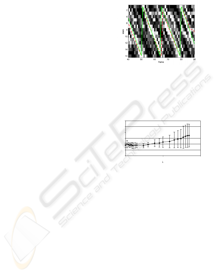
The algorithm was tested on 12 video clips of dif-
ferent people walking on a treadmill, an example of
the state probability matrix and calculated optimal
route is shown in Figure 2. There are only 16 states
as the number of phases was reduced by a half as dis-
cussed in Section 3. The lighter a box is the higher
the probability of that state. Notice there is very close
agreement between the extracted data and the ground
truth. The graph appears as a sawtooth due to the
cyclic nature of gait, once the last state is reached it
will then return back to the first state.
The average error in estimating gait phase as a func-
tion of λ is shown in Figure 3. All errors that are
used to quantify the accuracy of our method are cal-
culated as the average difference between the hand
Figure 2: Example of a state probability matrix, green solid
line shows ground truth, red dashed lines shows extracted
optimal path. The lighter a box the probable that state is.
labeled ground truth and the estimated gait phase (the
average difference between the red and green line in
Figure 2). Error bars show the calculated standard de-
viation of the errors for all the clips the algorithm was
tested on.
0
0.5
1
1.5
2
2.5
3
1 10 100
error/states per frame
Figure 3: Average error of gait phase estimation as a func-
tion of λ.
The lowest average error is when λ = 3.0, however
there is not much difference between this and when
λ = 1.0 implying the trajectories for each frame could
be classified independently to observations made in
previous frames. Figure 3 shows that the standard de-
viation of the results gets larger as λ increases, this
is because for a larger value of λ we assume a fea-
ture can only move into the next consecutive phase
for longer, meaning that the phase of the person be-
ing observed and that estimated by our model will be-
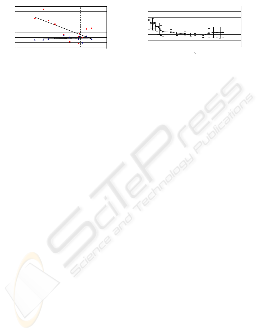
come offset. Consider the results shown in Figure 4,
the errors when λ = 2 appear independent of gait cy-
cle length, however when λ = 50 the error is generally
greater the bigger the difference between the length of
gait cycle of the walker and the model.
To visually demonstrate the accuracy of our method
a simple stick man model was created by learning
the average pose of each phase from the ground truth
data. Some sample frames are shown in Figure 6.
Our results show that when λ = 3.0 we are able to
achieve an average error in estimating the correct state
USING LOW-LEVEL MOTION TO ESTIMATE GAIT PHASE
499

0
0.5
1
1.5
2
2.5
3
3.5
0 0.2 0.4 0.6 0.8 1 1.2 1.4 1.6 1.8
log ( )
error/states per frame
0
0.5
1
1.5
2
2.5
3
3.5
4
22 24 26 28 30 32 34 36
average gait length/frames
error/states per frame
Figure 4: Error of gait phase estimation compared to gait
length; blue diamonds λ = 2.0, red squares λ = 50.0, the
dashed vertical line shows the number of phases in the
model.
of 0.9 ± 0.3 states per frame, this corresponds to a
temporal error of about 0.05 seconds.
To improve the generality of our algorithm we want
it to be able to work on people walking in real world
situations, these scenes will typically have more back-
ground clutter and as a result the tracking will contain
more errors. Unlike when people are walking on a
treadmill and have no net motion, people walking in
the real world have a translational motion in the direc-
tion they are walking. Our approach is to compensate
for this translation so that the walker is in a globally
stationary frame of reference.
We use a particle filter to propagate multiple hypoth-
esis of the position of the bounding box. We design
a likelihood function that will favour positions that
contain larger numbers of foreground points over po-
sitions that have fewer. After each frame we resam-
ple our distribution of particles so that those with low
likelihoods will typically be replaced by those with
higher likelihoods, we then propagate the particles
by allowing them to perform a random walk. Eight
frames are allowed to let the particle filter initialise
before phase estimation commences. We also use a
low pass filter to smooth the motion of the bounding
box.
To minimise the effect of foreground outliers we only
consider feature points that are located inside the
bounding box.
We tested this method on 6 clips of different people
walking in an outdoors scene. In three clips the cam-
era remained stationary and in the remaining clips the
camera panned to follow the person as they walked.
The error as a function of λ is shown in Figure 5. In
contrast to Figure 3 the error now initially decreases
as λ gets larger, this is as there are now additional
errors introduced through the estimation of the fore-
ground object’s motion, a larger λ is needed so that a
larger temporal window is used to integrate out errors.
When λ = 20 we obtain an average error of 0.9 ± 0.2
states per frame.
By learning a different pose for each gait phase we
0
0.5
1
1.5
2
2.5
3
3.5
1 10 100
error/states per frame
Figure 5: Average error of gait phase estimation as a func-
tion of λ.
have been able to crudely estimate pose. However
the poses that our system is capable of extracting is
limited to the number of phases in our model. These
estimates of pose could be used to initialise a further
search using methods such as deterministic optimisa-
tion (Urtasun et al., 2005) or dynamic programming
(Lan and Huttenlocher, 2004).
The height of the person used as ground truth was
about 380 pixels, the largest walker in our data set was
420 pixels in height and the smallest was 310 pixels in
height. This demonstrates that our approach can cope
with large changes in scale without having to adjust
the original models to compensate.
5 CONCLUSIONS
We have presented a system that is capable of robustly
and accurately estimating gait phase using the mo-
tion of a sparse set of feature points. This has been
achieved by building low-level motion models from
ground truth data obtained from a single person walk-
ing for 14 complete gait cycles. Despite this small
amount of training data our system has been shown
to be robust to changes in frequency, walker height
and gait characteristics. This has been achieved de-
spite a large amount of noise and uncertainty in the
observed tracking data. This work has demonstrated
the large amount of extractable information present in
low-level motion that is currently not being exploited.
The next step in the work is to integrate spatial infor-
mation to the models, so as well as being concerned
with how points move we consider where they move
relative to one another.
REFERENCES
Argawal, A. and Triggs, B. (2004). Tracking articulated
motion with piecewise learned dynamical models. In
ECCV, pages 54–65.
Caillette, F., Galata, A., and Howard, T. (2005). Real-Time
3-D Human Body Tracking using Variable Length
Markov Models. In BMVC, pages 469–478.
VISAPP 2008 - International Conference on Computer Vision Theory and Applications
500

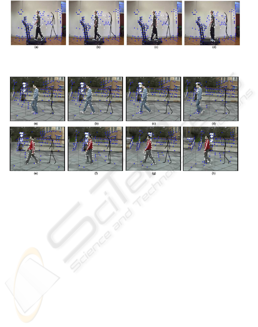
Figure 6: Sample frames with extracted phase illustrated by a stick man; white points represent KLT features classified as
foreground points, blue points represent KLT features classified as background points.
Figure 7: Figures (a) to (d) are frames taken from a sequence where the camera was stationary, Figures (e) to (g) are frames
taken from a sequence where the camera panned to follow the walker; white points represent KLT features classified as
foreground points, blue points represent KLT features classified as background points.
Coughlan, J., Yuille, A., English, C., and Snow, D. (2000).
Efficient deformable template detection and localiza-
tion without user initialization. CVIU, 78(3):303–319.
Deutscher, J., Blake, A., and Reid, I. D. (2000). Articulated
body motion capture by annealed particle filtering. In
CVPR, pages 126–133.
Gibson, D., Campbell, N., and Thomas, B. (2003).
Quadruped gait analysis using sparse motion informa-
tion. In ICIP, pages 333–336.
Havasi, L., Szlavik, Z., and Sziranyi, T. (2007). Detection
of gait characteristics for scene registration in video
surveillance system. IEEE Trasactions on Image Pro-
cessing, 16(2):503–510.
Hu, S. and Buxton, B. F. (2005). Using temporal coher-
ence for gait pose estimation from a monocular cam-
era view. In BMVC, pages 449–558.
Lan, X. and Huttenlocher, D. P. (2004). A unified spatio-
temporal articulated model for tracking. In CVPR,
pages 722–729.
Micilotta, A. S., Ong, E. J., and Bowden, R. (2006). Real-
Time Upper Body Detection and 3D Pose Estimation
in Monoscopic Images. In ECCV, pages 139–150.
Navaratnam, R., Thayananthan, A., Torr, P., and Cipolla,
R. (2005). Hierarchical part-based human body pose
estimation. In BMVC, pages 479–488.
Schuldt, C., Laptev, I., and Caputo, B. (2004). Recognizing
human actions: A local svm approach. In ICPR, pages
32–36.
Shi, J. and Tomasi, C. (1994). Good features to track. In
CVPR, pages 593 – 600.
Sidenbladh, H., Black, M. J., and Fleet, D. J. (2000).
Stochastic Tracking of 3D Human Figures Using 2D
Image Motion. In ECCV, pages 702–718.
Song, Y., Goncalves, L., and Perona, P. (2001). Learning
probabilistic structure for human motion detection. In
CVPR, pages 771–777.
Urtasun, R., Fleet, D. J., Hertzmann, A., and Fua, P. (2005).
Priors for people tracking from small training sets. In
ICCV, pages 403–410.
USING LOW-LEVEL MOTION TO ESTIMATE GAIT PHASE
501