SIMPLE BUT EFFECTIVE TREE STRUCTURES FOR DYNAMIC

PROGRAMMING-BASED STEREO MATCHING

Michael Bleyer and Margrit Gelautz

Institute for Software Technology and Interactive Systems, Vienna University of Technology

Favoritenstrasse 9-11/188/2, A-1040 Vienna, Austria

Keywords:

Stereo matching, tree-based dynamic programming, fast stereo method.

Abstract:

This work describes a fast method for computing dense stereo correspondences that is capable of generating

results close to the state-of-the-art. We propose running a separate disparity computation process in each

image pixel. The idea is to root a tree graph on the pixel whose disparity needs to be reconstructed. The tree

thereby forms an individual approximation of the standard four-connected grid for this speciﬁc pixel. An exact

optimum of a predeﬁned energy function on the applied tree structure is determined via dynamic programming

(DP), and the root pixel is assigned to the disparity of optimal costs. We present two simple tree structures

that allow for the efﬁcient calculation of all trees’ optima with only four scanline-based DP passes. These

simple trees are designed to capture all pixels of the reference frame and incorporate horizontal and vertical

smoothness edges in order to weaken the scanline streaking problem inherent in DP-based approaches. We

evaluate our results using the Middlebury test set. Our algorithm currently ranks at the eighth position of

approximately 30 algorithms in the Middlebury database. More importantly, it is the currently best-performing

method that does not use image segmentation and is signiﬁcantly faster than most competing algorithms. Our

method needs less than a second to determine the disparity map for typical stereo pairs.

1 INTRODUCTION

Stereo vision represents an inexpensive way for re-

constructing three-dimensional information from the

surrounding environment and is therefore of vital

importance for a large number of vision applica-

tions. Unfortunately, the key step in stereo vision,

i.e. the stereo matching problem, cannot be regarded

as solved. Factors that complicate the matching pro-

cess include image noise, untextured regions and the

occlusion problem. Although there is a large body

of literature, choosing a stereo algorithm for a practi-

cal application is still difﬁcult. While state-of-the-art

methods are computationally rather demanding, fast

techniques generate signiﬁcantly worse results. This

paper proposes an algorithm that represents a good

compromise between these conﬂicting requirements.

Stereo techniques are commonly divided between

local and global methods. Local algorithms are com-

putationally cheap, but they can typically not com-

pete with state-of-the-art results. We therefore fo-

cus our discussion on the latter category. A more

complete review of stereo methods is, however, given

in (Scharstein and Szeliski, 2002).

Global algorithms transform the stereo matching

task into an optimization problem. They seek for a

disparity map D that minimizes a predeﬁned energy

functional E(D), which is typically in the form of

E(D) = E

data

(D) + E

smooth

(D). (1)

Here, the data term E

data

assesses the agreement

of the disparity solution with the input images by

computing a match measurement. In addition, the

smoothness term E

smooth

imposes a penalty on spa-

tially neighbouring pixels carrying different disparity

labels. This term is motivated by the fact that neigh-

bouring image points are highly correlated, i.e. they

are likely to have similar disparities. A natural choice

for a pixel’s neighbourhood is the four-connected

neighbourhood structure, so that a pixel’s disparity is

biased towards the disparities of its closest two hori-

zontal and two vertical neighbours. This neighbour-

hood system leads to the standard four-connectedgrid

shown in Figure 1a.

Optimization of (1) is known to be NP-complete

for discontinuity-preserving smoothness functions.

Modern stereo techniques commonly apply graph-

cuts (Boykov et al., 2001) or belief propagation (Sun

et al., 2003) to approximate such energies. Meth-

ods that build upon these minimization schemes cur-

rently represent the state-of-the-art in stereo match-

415

Bleyer M. and Gelautz M. (2008).

SIMPLE BUT EFFECTIVE TREE STRUCTURES FOR DYNAMIC PROGRAMMING-BASED STEREO MATCHING.

In Proceedings of the Third International Conference on Computer Vision Theory and Applications, pages 415-422

DOI: 10.5220/0001072904150422

 SciTePress

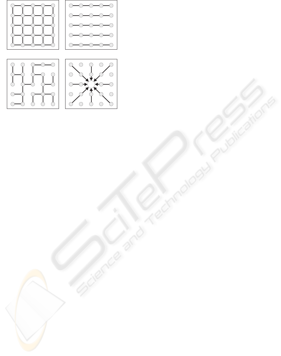
(a) (b)

Figure 1: Grid structures of previous approaches. Nodes

represent pixels, while edges indicate that the smooth-

ness function operates on the adjacent nodes. (a) Four-

connected grid. (b) Scanline-based DP approaches. (c)

Tree-based DP proposed by (Veksler, 2005). (d) Approach

of (Hirschm¨uller, 2005) to derive the disparity of pixel p.

ing (Scharstein and Szeliski, 2002). However, a se-

vere limitation of these optimization algorithms is that

they are computationally rather expensive. Especially

for the graph-cut approach, calculation of a single dis-

parity map can still take several minutes.

To bypass the NP-complete optimization problem,

classical DP approaches (Bobick and Intille, 1999;

Ohta and Kanade, 1985; Wang et al., 2006) adopt

a greatly simpliﬁed neighbourhood structure in their

smoothness terms. They enforce smoothness only

within, but not across horizontal scanlines. The corre-

sponding grid graph is illustrated in Figure 1b. Since

there is no interconnection between horizontal scan-

lines, an energy minimum for this grid structure can

be derived by computing the optimum for each scan-

line separately. The exact optimum of (1) on each in-

dividual scanline is then determined using DP. Such

approaches are favourable for their excellent com-

putational speed. Skipping the vertical smoothness

edges, however, leads to the well-known scanline

streaking effect. This inherent problem represents a

major reason for the bad reconstruction quality of DP

in comparison to the state-of-the-art.

Recently, (Veksler, 2005) proposed approximat-

ing the four-connected grid via a tree. The motiva-

tion is that efﬁcient DP-based optimization also works

on tree structures. Roughly spoken, the tree is con-

structed by discarding edges that show a high gradient

in the intensity image from the four-connected grid.

In contrast to scanline-based DP, horizontal and ver-

tical edges are treated symmetrically, which weakens

the streaking problem. Nevertheless, as can be seen

from Figure 1c, a large number of edges have to be

sacriﬁced in order to obtain a tree structure. The in-

formation of these edges remains unused, which is

most likely the reason for the only average results

of this method. Subsequent work (Deng and Lin,

2006; Lei et al., 2006) combines tree-based DP with

colour segmentation. These algorithms improve the

results on standard images such as the Middlebury

set (Scharstein and Szeliski, 2002). They, however,

fail if segments overlap disparity discontinuities.

A different approach to handle the streaking prob-

lem is to compute multiple DP passes. Two-pass

methods (Gong and Yang, 2005; Kim et al., 2005)

ﬁrst apply DP on the horizontal scanlines and use the

results to bias the second pass, which operates on

the vertical scanlines. While horizontal streaks are

reduced, these algorithms introduce vertical streaks,

and their scanline-based nature is clearly visible in the

resulting disparity maps.

(Hirschm¨uller, 2005) proposed a hybrid approach

between local and global methods. The disparity

of each pixel is computed using the winner-takes-all

strategy, i.e. without considering the disparity assign-

ments of neighbouring pixels. Instead of aggregating

matching costs from spatially surrounding pixels, the

algorithm computes DP paths from various directions

towards each pixel p as shown in Figure 1d. Cost

aggregation is then performed by summing up the in-

dividual path costs. In Hirschm¨uller’s approach, the

disparity of an image point is inﬂuenced by only a

small subset of the whole image’s pixels. This repre-

sents a problem if none of the paths captures enough

texture to provide a clear cost minimum at the correct

disparity. To weaken this problem, Hirschm¨uller pro-

posed increasing the number of paths. Nevertheless,

this results in higher computational demands and only

partially represents a remedy to the problem. In a sub-

sequent paper (Hirschm¨uller, 2006), he addressed this

problem using image segmentation.

2 THE SIMPLE TREE METHOD

The algorithm proposed in this paper performs a sep-

arate disparity computation for each individual pixel.

We apply an individual tree construction in order to

determine the disparity of a single pixel. The tree’s

root node is formed by the pixel whose disparity

needs to be computed. Although our trees prove to be

effective, their structure is relatively simple. (Hence,

we call our algorithm the Simple Tree Method.) For

now, it is only important to know that a tree spans all

pixels of the reference frame. A global minimum of

VISAPP 2008 - International Conference on Computer Vision Theory and Applications

416

an energy function that operates on the tree structure

is determined via DP. We then look up the disparity

that lies on this energy minimum in the root node. Fi-

nally, this disparity is assigned to the image point for

which we performed the disparity computation.

In comparison to (Hirschm¨uller, 2005), our algo-

rithm assigns disparities based on the exact solution

of a clearly deﬁned optimization problem. This might

represent a more “meaningful” result than selecting

the minimum of summed-up path costs. More impor-

tantly, we use tree structures that incorporateall pixels

of the reference image. A pixel’s disparity is there-

fore inﬂuenced by all other pixels and not just by a

subset thereof. This is what (Veksler, 2005) refers to

as “truly global”. Practically spoken, our algorithm

does not show the problem of missing image features

that help to disambiguate a pixel’s disparity, which is

speciﬁcally important in less textured image regions.

In the context of (Veksler, 2005), the most distinct

difference is that we do not apply a single tree to com-

pute the disparities of all pixels at once, but design

more ﬂexible trees that vary their grid structures with

the spatial position of the pixel under consideration.

Obviously, we also share the disadvantage of losing

a large number of edges by approximating the four-

connected grid via a tree. However, as will be shown

in this section, we address this problem by using two

complementary tree structures, each of which incor-

porating a complementary set of edges.

The remainder of this section is organized as fol-

lows. We start by deﬁning our energy function (sec-

tion 2.1). We then present the tree structures applied

in our approach (section 2.2). DP on a tree is reviewed

in section 2.3. Efﬁcient optimization of the energy

function on our tree structures is discussed in section

2.4. Section 2.5 shows how our algorithm combines

two different types of trees. Finally, occlusion han-

dling is addressed in section 2.6.

2.1 Energy Function

Let I be the set of all pixels in the reference frame

and D denote the set of allowed disparity labels. We

formulate the stereo matching task as ﬁnding a dis-

parity solution D that maps each pixel p ∈ I to a dis-

parity d

∈ D . The goodness of a disparity map D is

evaluated by an energy functional, which is subject to

minimization. We deﬁne the energy function by

E(D) =

∑

p∈I

m(p, d

) +

∑

(p,q)∈N

s(d

, d

). (2)

Here, the data term m(p, d

) computes the pixel dis-

similarity of p being assigned to d

. We implement

this function using the sampling-insensitive measure-

p p

(a) (b)

Figure 2: Tree-based approximations of the four-connected

grid applied in this approach. Two trees are constructed for

each pixel p of the reference frame. (a) Horizontal Tree. (b)

Vertical Tree.

ment of (Birchﬁeld and Tomasi, 1998) on RGB val-

ues. The smoothness function applied on two pixels

p and q that are neighbours according to a predeﬁned

set N is deﬁned by

s(d

, d

) =







0 : d

= d

: |d

− d

| = 1

: otherwise.

(3)

We impose a user-deﬁned penalty P

for small jumps

in disparity that do not exceed a value of one pixel.

Such jumps commonly occur for slanted surfaces and

are typically overpenalized when using the standard

Potts model. A second penalty P

with P

> P

ac-

counts for penalizing large jumps in disparity that oc-

cur at disparity borders. In order to align disparity dis-

continuities with discontinuities in the intensity im-

age, we compute the value of P



· P

′

: |I

− I

| < T

′

: otherwise

(4)

with |I

− I

| being the summed-up absolute differ-

ences of RGB channels. P

′

, P

and T denote prede-

ﬁned constants.

2.2 Simple Tree Structures

Choosing the set of neighbours N in equation (2)

deﬁnes the complexity of the resulting optimization

problem. In the ideal case, N is formed by all pairs of

spatially neighbouring pixels of the reference image.

Since it is known that optimization of the resulting

four-connected grid (Figure 1a) is difﬁcult and com-

putationally challenging, we propose ﬁnding approx-

imations of this grid in each individual image point.

Our approximationsare based on trees, i.e. graphs that

do not contain cycles. If N consists of pixel pairs that

form a tree on the grid graph, exact minimization of

our energy can efﬁciently be accomplished via DP.

Our ﬁrst approximation is shown in Figure 2a.

The tree is rooted on pixel p whose disparity is com-

puted. It includes all horizontal smoothness edges

SIMPLE BUT EFFECTIVE TREE STRUCTURES FOR DYNAMIC PROGRAMMING-BASED STEREO MATCHING

417

of the four-connected grid. In addition, the edges

from the vertical scanline on which p is located en-

force smoothness in vertical direction. Since horizon-

tal edges dominate in this tree structure, we refer to

this tree as the Horizontal Tree.

The second approximation illustrated in Figure

2b can be regarded as the complementary tree struc-

ture to the Horizontal Tree. The idea is to include

those edges that have been discarded from the four-

connected grid in order to derive the Horizontal Tree.

The tree is formed by all vertical edges as well as the

edges of the horizontal scanline on which p resides.

We call this tree the Vertical Tree.

To determine p’s disparity, we optimize our en-

ergy function with the set N being built by all edges

of the tree rooted on p. The disparity d

is then de-

rived by selecting the disparity that lies on the com-

puted optimum. Our algorithm thereby combines the

results of Horizontal and Vertical Trees. Section 2.5

shows how this is accomplished.

2.3 DP on a Tree

We can determine an exact optimum of energy (2) on

a tree via DP. This works as follows. Let r be the

root node of a tree. A minimum value of energy for

r at disparity d is computed by passing r and d as

arguments to a recursive function l() deﬁned by

l(p, d) = m(p, d) +

∑

q∈v(p)

min

i∈D

(s(d,i) + l(q, i)). (5)

Here, the function v(p) returns the siblings of p, i.e.

the nodes that have p as their direct predecessor on

the path to the root r. Since, by deﬁnition, leaf nodes

do not have siblings, the function l() can be directly

evaluated for these nodes. For a non-leaf node, l()

is evaluated when the values of l() have been com-

puted for all its siblings. The algorithm terminates

once it reaches the root r. A global energy minimum

is computed by min

d∈D

l(r, d), and r’s disparity is de-

termined by argmin

d∈D

l(r, d).

(Veksler, 2005) has shown that for her energy

function the complexity of this algorithm can be re-

duced to O(|D |wh) with w and h being the image

width and height. However, if we apply the algorithm

on a large number of trees, this can easily become

computationally intractable.

2.4 DP on Simple Trees

In our approach, we beneﬁt from the simple struc-

ture of our trees to signiﬁcantly improve the compu-

tational speed. We show how the optima of all Hori-

zontal Trees are determined with four scanline-based

wy,

x y,

1,y

(a)

wy,

1,y

x y,

(b)

wy,

1,y

x y,

(c)

Figure 3: Computation of optimal costs on a scanline. Ar-

rows determine the order in which path costs are computed.

In the tree DP algorithm, r denotes the position of the root

node. (a) Forward pass. (b) Backward pass. (c) Optimal

costs for pixel p

x,y

are derived by combining costs of for-

ward and backward passes.

DP passes. An analogous construction can be applied

for Vertical Trees.

In the ﬁrst step, we optimize horizontal scanlines

separately from each other. The goal is to compute

the values of an array C with C[p, d] representing the

costs of an optimal disparity solution in which pixel p

is assigned to disparity d. In this context, an optimal

disparity solution is one that minimizes the energy on

individual scanlines. In the following, the values of C

are determined with two DP passes as shown in Figure

3. C is needed for further processing.

The ﬁrst DP pass, which is referred to as forward

pass, is similar to that of standard DP methods. We

compute the optimal costs for reaching each pixel’s

disparity from the leftmost pixel of a scanline. These

costs are calculated using the following recursion,

which represents a simpliﬁed form of equation (5):

′

(p, d) = m(p, d) + min

i∈D



s(d, i) + l

′

(q, i)



. (6)

Here, q denotes the sibling of p. For the forward pass,

this is the pixel to the left of p. In contrast to stan-

dard DP methods, l() does not enforce the ordering

constraint. This approach is therefore closer related

to Scanline Optimization (Scharstein and Szeliski,

2002). The accumulated costs l

′

(p, d) for each pixel

p and disparity d are recorded in an array F.

As a second DP pass, the backward pass deter-

mines the costs to reach each pixel’s disparity from

the rightmost pixel of a scanline. These costs are com-

puted using the function l

′

(p, d) with p’s sibling q be-

ing deﬁned as the pixel to the right of p. An array B

stores the accumulated costs of the backward pass.

The optimal costs for each pixel’s disparity can be

computed from the accumulated costs of forward and

backward passes (Kim et al., 2005). Let p

x,y

denote

the pixel at coordinates (x, y). The energy minimum

VISAPP 2008 - International Conference on Computer Vision Theory and Applications

418

x,y

wy,

1,y

x,1

x h,

Figure 4: Computation of optimal costs on the Horizontal

Tree rooted on pixel p

x,y

. DP only needs to be performed

for solid arrows. Optimal values are determined by DP on

the vertical scanline using precomputed path costs.

of p

x,y

at disparity d is derived by expanding the sum

in equation (5) at pixel p

x,y

, i.e.

C(p

x,y

, d) = m(p

x,y

, d) + min

i∈D

(s(d, i) + F[p

x−1,y

, i])

+ min

i∈D

(s(d, i) + B[p

x+1,y

, i]).

(7)

This is equivalent to

C(p

x,y

, d) = F[p

x,y

, d] + B[p

x,y

, d] − m(p

x,y

, d). (8)

It is noteworthy that min

d∈D

C[p, d] is constant for all

pixels p of the same scanline. This makes sense, since

this value represents the global optimum of our en-

ergy function on the scanline. Given that this opti-

mum is unique, we can reconstruct the optimal dispar-

ity assignment by computing d

= argmin

d∈D

C[p, d].

In the following, we calculate the energy minima

for all Horizontal Trees. The basic idea is sketched in

Figure 4. We compute the values of an array H with

H[p, d] being the energy optimum for the Horizontal

Tree rooted on pixel p at disparity d. This value is

derived by passing p and d as parameters to a function

′′

(). Considering the special structure of the tree, we

deﬁne l

′′

() by expanding the sum in equation (5):

′′

x,y

, d) = m(p

x,y

, d) + min

i∈D

(s(d, i) + F[p

x−1,y

, i])

+ min

i∈D

(s(d, i) + B[p

x+1,y

, i])

∑

q∈v

′

x,y

)

min

i∈D



s(d, i) + l

′′

(q, i)



(9)

Here, the function v

′

(p) returns the siblings that are

connected to their predecessor via a vertical edge. We

use the precomputed values of array C to write

′′

x,y

, d) = C[p

x,y

, d]

∑

q∈v

′

x,y

)

min

i∈D



s(d, i) + l

′′

(q, i)



(10)

In the computation of H[p, d] for each pixel p and

disparity d, we take advantage of the fact that l

′′

()

solely operates on pixels of the same vertical scan-

line. When interpreting the values of C as the match-

ing costs m() of a DP path, this calculation is, in

fact, equivalent to scanline-based DP along the ver-

tical scanlines. Hence, we can use the same strategy

as before. That is, we compute forward and backward

passes on the precomputed values of C in vertical di-

rection. Finally, the forward and backward passes are

combined to determine the energy minima in H.

Computation of the array V representing the op-

tima for the Vertical Tree structure is accomplished

equivalently, except that we ﬁrst optimize vertical

scanlines and then operate on the horizontal ones.

Regarding the computational performance, the

most expensive part of our algorithm is the calcu-

lation of scanline-based DP passes. In a naive im-

plementation, evaluation of l

′

(p, d) in equation (6)

for each pixel p and disparity d takes a complex-

ity of O(|D |

wh). This is an undesirable prop-

erty when designing a fast algorithm. Analogously

to (Hirschm¨uller, 2005), we reformulate l

′

() for our

energy function as

′

(p, d) =m(p, d) + min(l

′

(q, d), l

′

(q, d − 1) + P

′

(q, d + 1) + P

, min

i∈D

′

(q, i) + P

(11)

Let us compute the values of l

′

(p, d) at a speciﬁc

pixel p for each disparity d ∈ D using this formula-

tion. The value of min

i∈D

′

(q, i) can be precomputed,

so that the complexity of this operation is linear in the

number of disparity labels. Consequently, the overall

complexity of a DP pass is reduced to O(|D |wh).

2.5 Combining the Tree Structures

To combine Horizontal and Vertical Trees in our algo-

rithm, we propose the following strategy. We start by

operating on the Vertical Tree structure and determine

the array V as described in section 2.4. V serves to

propagate the results of the Vertical Tree computation

to the subsequent calculation of Horizontal Trees. We

therefore manipulate the data costs m(). The updated

matching scores m

′

() are derived by

′

(p, d) = m(p, d) + λ · (V(p, d) − min

i∈D

V(p, i))

(12)

with λ being a parameter that regulates the inﬂuence

of the Vertical Trees on the ﬁnal disparity map. Our

update proceduremeasures the difference between the

costs of the solution in which a pixel p is assigned to

disparity d and the costs of p’s optimal disparity as-

signment. If d does not represent an optimal disparity

SIMPLE BUT EFFECTIVE TREE STRUCTURES FOR DYNAMIC PROGRAMMING-BASED STEREO MATCHING

419

for p, we impose a penalty on d. The amount of this

penalty is proportional to the computed difference. If

the difference is large, it is likely that d is the wrong

disparity for pixel p. This information is passed to the

subsequent calculation by imposing a large penalty.

However, if there are pixels whose costs are not much

higher than those of the optimal disparity or the opti-

mal disparity is not unique, estimation of p’s dispar-

ity is still ambiguous. Such disparities receive only a

small penalty, and it is left to the subsequent compu-

tation of Horizontal Trees to resolve this ambiguity.

The updated matching scores then represent the

input to the calculation of Horizontal Trees. We de-

termine the values of the array H using the modiﬁed

data costs m

′

(). The ﬁnal disparity for each pixel p is

then selected by d

= argmin

d∈D

H[p, d].

2.6 Occlusion Handling

An inherent problem in stereo matching is that of oc-

cluded pixels, i.e. pixels visible in one input image,

but not in the other one. We cannot expect that our

algorithm generates correct depth information in the

absence of a matching point. Even worse, the smooth-

ness term of our energy function corrupts disparity es-

timates for non-occludedpixels by propagatingwrong

disparity information gathered in occluded regions.

To handle occlusions, we compute two disparity

maps. The ﬁrst disparity map D

is calculated with

the right frame being the reference image. D

serves

solely to identify the occluded pixels of the left image.

We use D

to warp the right image into the geometry

of the left view. Pixels of the warped image that do

not receive contribution from at least one pixel of the

right image are marked as being occluded (Bleyer and

Gelautz, 2005). These pixels are recorded in an occlu-

sion map for the left image denoted by O

. We post-

process O

by deleting occluded pixels whose left and

right spatial neighbours are marked as non-occluded.

Such pixels typically occur for slanted surfaces that

are oversampled in the left image (Ogale and Aloi-

monos, 2004). These pixels are not occluded, but vi-

olate the uniqueness constraint.

The second disparity map D

is computed with the

left image being the reference frame. At this point, we

do not attempt to assign occluded pixels of O

to “cor-

rect” disparities. We, however, attempt to avoid that

occluded pixels of O

propagate wrong disparities.

We therefore extend the smoothness term of equation

(3) by an additional constraint. This constraint is: If

at least one of the two neighbouring pixels is marked

as occluded in O

, the smoothness penalty is set to

zero. As a consequence, an occluded pixel does not

inﬂuence the disparity assignments of its neighbour-

ing pixels by imposing the smoothness penalty.

The ﬁnal disparity map of our algorithm is de-

rived from D

by overwriting the estimated disparities

for occluded pixels with more “meaningful” disparity

values. For each occluded pixel p in the occlusion

map O

, we search p’s closest non-occluded pixels

on the same horizontal scanline in left and right di-

rections. We determine the minimum of both pixels’

disparities and assign this disparity to p.

3 EXPERIMENTAL RESULTS

We use the Middlebury data set (Scharstein and

Szeliski, 2002) to evaluate the results of our algo-

rithm. The test set consists of four stereo pairs for

which ground truth data is provided. Results of our

algorithm on these stereo images are shown in Fig-

ure 5. All disparity maps have been generated using

constant parameter settings. (The parameters are set

to P

= 20, P

′

= 30, P

= 4, T = 30 and λ = 0.025.)

Obviously, we could improve the results by tuning the

parameters for each image pair separately.

The disparity maps in Figure 5 show that our al-

gorithm produces smooth disparity results. Due to

the occlusion handling procedure and the algorithm’s

pixel-based nature, disparity discontinuities appear to

be correctly captured. The algorithm also preserves

details in the disparity map (e.g., sticks in the cup

of the Cones data set). As opposed to other DP ap-

proaches, our disparity maps seem to be almost free of

streaks. This can be attributed to the structure of our

trees that captures horizontal and vertical smoothness

edges. Our disparity maps also hardly contain iso-

lated pixels. These are typical artefacts produced by

the Semi-Global Approach of (Hirschm¨uller, 2005)

when the DP paths do not capture enough texture.

Our approach avoids this problem by applying trees

that span all pixels of the reference image. A rela-

tively large error is, however, found to the right of the

pink teddy in the Teddy data set. This region is virtu-

ally free of texture and image noise biases the results

towards the wrong disparity.

We use the Middlebury stereo website (Scharstein

and Szeliski, 2002) for a quantitative comparison

against competing approaches. Currently, our algo-

rithm ranks on the eighth position of approximately

30 algorithms in the Middlebury online table. Most

methods that achieve a better ranking build on graph-

cuts or belief propagation. They are far slower than

the proposed algorithm, which makes a compari-

son partially unfair. Moreover, all of the better-

performing techniques apply colour segmentation and

most of them use the segmentation information as a

VISAPP 2008 - International Conference on Computer Vision Theory and Applications

420

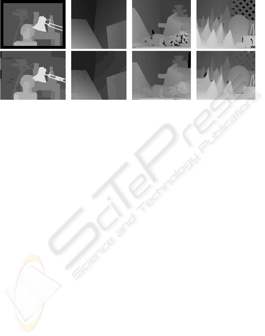
Figure 5: Results of our algorithm on the Tsukuba, Venus, Teddy and Cones image pairs from the Middlebury data set. The

upper row shows the ground truth images. The bottom row shows the disparity maps computed by the Simple Tree Method.

hard constraint. While segmentation works well on

the Middlebury data set, these algorithms fail in situa-

tions such as shown in Figure 6. Applying colour seg-

mentation on the reference image (Figure 6a) leads to

segments that overlap disparity discontinuities. Due

to these overlapping regions, the segmentation-based

algorithm of (Bleyer and Gelautz, 2005), which is

one of the top-performersin the Middlebury database,

generates erroneous disparity estimates in the proxim-

ity of disparity borders (Figure 6c). In contrast to this,

the proposed algorithm can correctly capture the dis-

parity discontinuities as the consequence of its pixel-

based nature (Figure 6d).

Table 1 gives a quantitative comparison of our

algorithm against other DP approaches. These re-

sults are obtained from the Middlebury website. Two

methods that apply colour segmentation show slightly

better results. Apart from the above described prob-

lem, it should be noted that performing image seg-

mentation (commonly accomplished using the mean-

shift algorithm) is also a computationally costly oper-

ation, which can spoil the speed advantage of DP op-

timization. (Lei et al., 2006) report running times be-

tween 10 and 25 seconds on the Middlebury data set

with most of the time being consumed by the segmen-

tation overhead. (Hirschm¨uller, 2006) states that seg-

mentation increases the running time of this approach

by 30–50 percent, which makes it likely that also this

method is slower than the proposed approach. It can

be seen from the table that our technique shows better

quantitative results than the Semi-Global Approach

of (Hirschm¨uller, 2005) and signiﬁcantly outperforms

the tree DP method of (Veksler, 2005).

We have run our method on a machine equipped

with two dual-core AMD Opteron processors clocked

at 2.4 GHz. To take advantage of this multi-core

architecture, we have parallelized the optimization

component of our algorithm. We therefore divide the

image into even sets of scanlines. The scanline sets

are then distributed among the CPUs for perform-

ing DP. Overall running times of our implementation

range from 0.18 seconds on the Tsukuba stereo pair

(384×288 pixels, 16 disparity labels) to 0.57 seconds

on the Teddy and Cones sets (450×375 pixels, 60 dis-

parity labels). It is realistic to expect real-time perfor-

mance as the result of further parallelization, which

can, for example, be implemented on the GPU.

4 CONCLUSIONS

The idea of this paper has been to generate a dense

disparity map by solving an individual optimization

problem for each image point. We approximate the

standard four-connected grid in each pixel of the ref-

erence frame. Our approximations build on two com-

plementary tree structures, i.e. the Horizontal Tree

and the Vertical Tree. We have shown that by ex-

ploiting the simple structure of these trees we can efﬁ-

ciently compute the exact solutions of all optimization

tasks with only few scanline-based DP passes.

Our algorithm produces disparity maps that are

almost free of the streaking problem inherent to DP

approaches. Currently, the method is the overall

best-performing algorithm in the Middlebury online

database that does not apply segmentation. Our algo-

rithm is faster than most competing methods, which

typically rely on graph-cuts or belief propagation. We

therefore see our algorithm as an alternative method

when speed matters. It takes less than a second to

compute the disparity map for typical image pairs.

SIMPLE BUT EFFECTIVE TREE STRUCTURES FOR DYNAMIC PROGRAMMING-BASED STEREO MATCHING

421

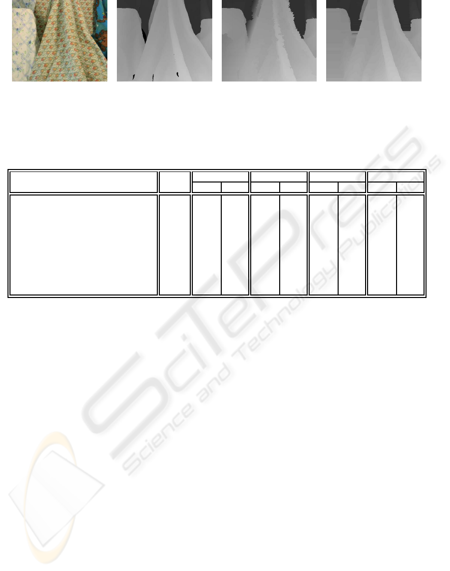
(a) (b) (c) (d)

Figure 6: Limitations of segmentation-based methods. (a) Reference view. (b) Ground truth. (c) Result of the segmentation-

based algorithm in (Bleyer and Gelautz, 2005). (Percentage of pixels having an absolute disparity error > 1 in non-occluded

regions = 4.08.) (d) Result of the proposed method. (Error percentage = 1.80.) More information is given in the text.

Table 1: Rankings of DP approaches in the Middlebury database. Values represent error percentages measured in different

image regions. Our algorithm (SimpleTree) is currently the overall best-performing method that does not use segmentation.

Algorithm Rank

Tsukuba Venus Teddy Cones

nocc all nocc all nocc all nocc all

C-SemiGlob (Hirschm¨uller, 2006) 5 2.61 3.29 0.25 0.57 5.14 11.8 2.77 8.35

RegionTreeDP (Lei et al., 2006) 6 1.39 1.64 0.22 0.57 7.42 11.9 6.31 11.9

SimpleTree 8 1.86 2.56 0.42 0.76 7.31 12.7 4.00 9.74

SegTreeDP (Deng and Lin, 2006) 10 2.21 2.76 0.46 0.60 9.58 15.2 3.23 7.86

SemiGlob (Hirschm¨uller, 2005) 12 3.26 3.96 1.00 1.57 6.02 12.2 3.06 9.75

RealTimeGPU (Wang et al., 2006) 19 2.05 4.22 1.92 2.98 7.23 14.4 6.41 13.7

ReliabilityDP (Gong and Yang, 2005) 21 1.36 3.39 2.35 3.48 9.82 16.9 12.9 19.9

TreeDP (Veksler, 2005) 22 1.99 2.84 1.41 2.10 15.9 23.9 10.0 18.3

DP (Scharstein and Szeliski, 2002) 24 4.12 5.04 10.1 11.0 14.0 21.6 10.5 19.1

SO (Scharstein and Szeliski, 2002) 27 5.08 7.22 9.44 10.9 19.9 28.2 13.0 22.8

ACKNOWLEDGEMENTS

This work has been supported by the Austrian Science

Fund (FWF) under project P19797.

REFERENCES

Birchﬁeld, S. and Tomasi, C. (1998). A pixel dissimilarity

measure that is insensitive to image sampling. TPAMI,

20(4):401–406.

Bleyer, M. and Gelautz, M. (2005). A layered stereo match-

ing algorithm using image segmentation and global

visibility constraints. ISPRS Journal, 59(3):128–150.

Bobick, A. and Intille, S. (1999). Large occlusion stereo.

IJCV, 33(3):181–200.

Boykov, Y., Veksler, O., and Zabih, R. (2001). Fast approx-

imate energy minimization via graph cuts. TPAMI,

23(11):1222–1239.

Deng, Y. and Lin, X. (2006). A fast line segment based

dense stereo algorithm using tree dynamic program-

ming. In ECCV, volume 3, pages 201–212.

Gong, M. and Yang, Y. (2005). Near real-time reliable

stereo matching using programmable graphics hard-

ware. In CVPR, pages 924–931.

Hirschm¨uller, H. (2005). Accurate and efﬁcient stereo pro-

cessing by semi-global matching and mutual informa-

tion. In CVPR, volume 2, pages 807–814.

Hirschm¨uller, H. (2006). Stereo vision in structured en-

vironments by consistent semi-global matching. In

CVPR, volume 2, pages 2386–2393.

Kim, J., Lee, K., Choi, B., and Lee, S. (2005). A dense

stereo matching using two-pass dynamic program-

ming with generalized ground control points. In

CVPR, volume 2, pages 1075–1082.

Lei, C., Selzer, J., and Yang, Y. (2006). Region-tree based

stereo using dynamic programming optimization. In

CVPR, volume 2, pages 2378–2385.

Ogale, A. S. and Aloimonos, Y. (2004). Stereo correspon-

dence with slanted surfaces: critical implications of

horizontal slant. In CVPR, pages 568–573.

Ohta, Y. and Kanade, T. (1985). Stereo by intra- and inter-

scanline search. TPAMI, 7(2):139–154.

Scharstein, D. and Szeliski, R. (2002). A taxon-

omy and evaluation of dense two-frame stereo cor-

respondence algorithms. IJCV, 47(1/2/3):7–42.

http://www.middlebury.edu/stereo/.

Sun, J., Zheng, N., and Shum, H. (2003). Stereo matching

using belief propagation. TPAMI, 25(7):787–800.

Veksler, O. (2005). Stereo correspondence by dynamic pro-

gramming on a tree. In CVPR, pages 384–390.

Wang, L., Liao, M., Gong, M., Yang, R., and Nister, D.

(2006). High quality real-time stereo using adap-

tive cost aggregation and dynamic programming. In

3DPVT.

VISAPP 2008 - International Conference on Computer Vision Theory and Applications

422