AN INVERSE MODEL FOR LOCALIZATION OF
LOW-DIFFUSIVITY REGIONS IN THE HEART USING ECG/MCG
SENSOR ARRAYS
Ashraf Atalla and Aleksandar Jeremic
Department of Electrical and Computer Engineering, McMaster University, Hamilton, ON Canada
Keywords:
Biological system modeling, diffusion equations, parameter estimation.
Abstract:
Cardiac activation and consequently performance of the heart can be severely affected by certain electrophysi-
ological anomalies such as irregular patterns in the activation of the heart. Since the wavefront propagation oc-
curs through the diffusion of ions (Na
+
,K
+
, etc.) the reduced mobility of ions can be equivalently represented
as a reduction of ionic diffusivity causing irregularities in heartbeats. In this paper we propose models for the
cardiac activation using inhomogeneous reaction-diffusion equations in the presence of diffusivity disorders.
We also derive corresponding statistical signal processing algorithms for estimating (localizing) parameters
describing these anomalies. We illustrate applicability of our techniques and demonstrate the identifiability of
the parameters through numerical examples using a realistic geometry.
1 INTRODUCTION
The phases of myocardial action potentials and pro-
cesses of myocardial depolarization and repolariza-
tion are well studied and described in most handbooks
of electrophysiology and electrocardiography (Gulra-
jani, Malmivuo). The underlying processes control-
ling the (re)polarization in the cardiac activation can
be described, on a molecular level, as diffusion of
ions through various channels (Na, K, etc.) giving
a rise to ionic current which in turn creates electro-
magnetic field on the torso surface which can be ex-
ternally measured.
Modeling the cardiac activation on a cellular level
(Gulrajani) has been a subject of considerable re-
search interest resulting in numerous models related
to membrane potential (e.g. Hodgkin-Huxley model).
However, these models are mainly suitable for for-
ward modeling in which the cardiac activation is sim-
ulated using a priori knowledge of various param-
eters. Complimentary to this approach is inverse
modeling in which information on cardiac activation
(and some physiological parameters) is deduced from
ECG/MCG measurements.
One of the most important parameters controlling
the activation wavefront propagation is the diffusiv-
ity (i.e., mobility of ions). Namely, significant loss of
ionic mobility can cause occurrence of irregular acti-
vation patterns and lead to various pathological con-
ditions such as arrhythmia, early after-depolarization,
etc. From a physiological point of view, these changes
usually occur due to ion depletion from a particular
region of the heart. As a result, the diffusivity in this
region becomes very small preventingthe propagation
of the activation wavefront and causing the aforemen-
tioned irregular patterns. Therefore, any algorithm
capable of detecting these anomalies can potentially
be useful to predict the onset of these cardiac phys-
iopathologies.
In this paper we propose a new activation model based
on the diffusion equation. Although the FitzHugh-
Nagumo model is based on the diffusion equation
its applicability to inverse approach and real data is
limited because of its isotropic and homogeneous na-
ture. In Section 2 we develop cardiac activation model
based on the reaction-diffusion equation with non-
homogeneous and anisotropic diffusion tensor. Such
a model can be used for detecting different physiolog-
ical conditions such as conductivity anomalies, which
can predate onset of various pathological conditions
such as cardiac arrhythmia, early after-depolarization,
etc. In Section 3 we derive the statistical and measure-
ments model using Geselowitz equations correspond-
ing to our diffusion based source. Using these models
we derive the generalized least squares (GLS) estima-
tor for localizing conductivity anomalies/disorders. In
Section 5 we demonstrate the applicability of our re-
sults using numerical simulations and in Section 6 we
present conclusions.
508
Atalla A. and Jeremic A. (2008).
AN INVERSE MODEL FOR LOCALIZATION OF LOW-DIFFUSIVITY REGIONS IN THE HEART USING ECG/MCG SENSOR ARRAYS.
In Proceedings of the First International Conference on Bio-inspired Systems and Signal Processing, pages 508-512
DOI: 10.5220/0001070005080512
Copyright
c
 SciTePress

2 PHYSICAL MODEL
During the spread of activation in the heart, the most
significant bioelectric source is the large potential dif-
ference that exists across the moving wavefront that
divides active (depolarized) from resting tissue. It
has been proposed that the cardiac excitation can be
modeled using reaction diffusion systems i.e., a set of
nonlinear partial differential equations (Panfilov and
Holden, 1997)
∂u
i
∂t
= f
i
(u) + ∇ · (D
i
∇u
i
) i = 1,...n (1)
where u = [u
1
,...u
n
]
T
is the state variable vector, f
i
are excitations, and D
i
diffusion tensors. Although
the above models can be used to model the propa-
gation even down to a cellular level, in order to de-
velop an inverse model a simplified approach similar
to (FitzHugh, 1961),(Rogers and McCulloch, 1994)
is needed. Therefore, we propose a reaction diffusion
model consisting of two state variables but with spa-
tially dependent diffusivity tensor
∂u
1
(r,t)
∂t
= ∇· (D(r)∇u
1
(r,t)) +
+g
T
(u(r,t))A
1
g(u(r,t))
∂u
2
(r,t)
∂t
= u
T
(r,t)A
2
u(r,t)
g(u(r,t)) = [u
2
1
(r,t),u
1
(r,t),u
2
(r,t),1]
T
where u
1
is the activation potential and u
2
is the rest-
ing potential.
The above model is the generalization of the ex-
isting models from at least two standpoints: a) by
allowing the diffusivity matrix to be spatially depen-
dent we can test for the presence of arbitrarily shaped
anomalies, and b) by adding higher-order polynomial
components we allow for wider range of dynamic be-
havior in the cardiac excitation. Note that in order to
apply the above model to the realistic geometry we
need to define boundary conditions. In our case we
impose ∂u
1
/∂n on the epicardial surface of the heart.
As for initial conditions, we define the active poten-
tial at time t = 0 as u
1
(r,0) = u
0
δ(r − r
0
) where δ()
is a Dirac delta function and r
0
is the activation point
in the myocardium. The initial condition for the inhi-
bition (u
2
) is set to zero.
To compute the electro-magnetic field on the torso
surface we utilize the Geselowitz (Geselowtiz, 1970)
equations that compute the potential φ(r,t) and mag-
netic field B(r,t) at a location r on the torso sur-
face at a time t from a given primary current distri-
bution J(r
′
,t) = ∇u
1
(r,t) within the heart.We use a
piecewise homogeneous torso model consisting of the
following surfaces: the outer torso, the inner torso,
and the heart. Therefore, we model the heart as a
volume G of M = 3 homogeneous layers separated
by closed surfaces S
i
,i = 1,. .. ,M. Let σ
−
i
and σ
+
i
be the conductivities of the layers inside and outside
S
i
respectively. We will denote by G
i
the regions
of different conductivities, and by G
M+1
the region
outside the torso, which behaves as an insulator i.e,
σ
−
M+1
= σ
+
M
= 0.
It has been shown that in the case of a piecewise
homogeneous torso model and using quasi-static as-
sumption the magnetic field at a location r and time
t is given by (Gulrajani, 1998) and (Malmivuo and
Plonsey, 1995)
B(r,t) = B
0
(r,t) +
µ
0
4π
M
∑
i=1
(σ
−
i
− σ
+
i
) ·
·
Z
S
i
φ(r
′
,t)
(r− r
′
)
kr − r
′
k
3
× dS(r
′
)
B
0
(r,t) =
µ
0
4π
Z
G
J(r
′
,t) × (r− r
′
)
kr − r
′
k
3
d
3
r
′
, (2)
where µ
0
is the magnetic permeability of the vacuum.
Similarly, the potential φ(r,t) is given by
(Geselowitz)
σ
−
k
+ σ
+
k
2
φ(r,t) = φ
0
(r)(σ
−
i
− σ
+
i
)+
+
1
4π
M
∑
i=1
(σ
−
i
− σ
+
i
)
Z
S
i
φ(r
′
,t)
(r− r
′
)
kr− r
′
k
3
· dS(r
′
),
φ
0
(r,t) =
1
4π
Z
G
J(r
′
,t) · (r− r
′
)
kr− r
′
k
3
d
3
r
′
,(3)
where we k is chosen so that r ∈ G
k
.
3 MEASUREMENT MODEL AND
STATISTICAL MODEL
In this section we introduce our parametric descrip-
tion of the diffusion anomaly and measurement noise
signals. To simplify the approach we assume that the
anomaly region can be modeled with an ellipsoid i.e.,
the region R of anomaly is given by
R = {r : (r− r
a
)
T
F(a,b,c,ψ,φ)
−1
(r− r
a
) ≤ 1}
where
F = T(φ,ψ)


a
2
0 0
0 b
2
0
0 0 c
2


T
T
(φ,ψ)
where a,b, c are the axes of anomaly ellipsoid, r
a
is
the center, and ψ and φ are the orientation parame-
ters (in 3D). The matrix T(φ,ψ) is the rotation matrix
AN INVERSE MODEL FOR LOCALIZATION OF LOW-DIFFUSIVITY REGIONS IN THE HEART USING
ECG/MCG SENSOR ARRAYS
509

given by
T(φ, ψ) =


cosφ sinφ 0
−sinφ cosφ 0
0 0 1


·


cosψ 0 sinψ
0 1 0
−sinψ 0 cosψ


(4)
The diffusion tensor is then
D(r) =

0 r ∈ R
D otherwise.
(5)
In the remainder of the myocardium tissue we assume
homogeneous but possibly anisotropic diffusion ten-
sor D.
Next, we assume that a bimodal array of n
B
MCG
and n
E
ECG sensors is used for the measurements.
Let n = n
B
+ n
E
. We assume that the sensors are lo-
cated at ρ
j
, j = 1,. .. ,n, and that time samples are
taken at uniformly spaced time points t
k
,k = 1,. ..,n
s
.
In addition, we assume that data acquisition is re-
peated n
c
times during several heart cycles in order
to improve the signal-to-noise (SNR) ratio. Then, the
n
s
-dimensional measurement vector of this array ob-
tained at time t
k
in the lth cycle is
y
lk
= f(θ,t
k
) + e
l
(t
k
), (6)
where y
lk
= [y
T
B
(t
k
),y
T
E
(t
k
)]
T
, θ is the collection of all
the parameters (a,b,c,r
0
,ψ,φ,u
0
,D,A
1
,A
2
) , f (θ,t
k
)
is the vector solution computed using finite elements,
and e
l
(t
k
) = [e
T
B
(t
k
),e
T
E
(t
k
)]
T
is additive noise. In the
remainder of the paper we omit the subscript l when-
ever it is obvious that the samples belong to the same
heart cycle. The subscripts B and E correspond to mag-
netic and electric components of the measurement
vector (noise), respectively. We further assume that
both magnetic and electric components of the noise
are zero-mean Gaussian, uncorrelated in space and
time with variances, σ
2
B
and σ
2
E
, respectively.
4 PARAMETER ESTIMATION
We first start by splitting the unknown parameters θ
into three groups: a) the unknown activation parame-
ters θ
0
= [u
0
,r
a
]
T
, and b) the unknown anomaly pa-
rameters θ
a
= [a,b,c,r
0
,φ,ψ]
T
. For simplicity in the
remainder of the paper we assume that the heart pa-
rameters
θ
h
= [vec(D),vec(A
1
1),vec(A
2
)]
T
(7)
where vec is the vector operator, are known. Note that
some in vitro studies (Sachse, 2004) suggest that these
parameters do not vary significantly between different
subjects and thus can be easily estimated using data
gathered from human subjects without any anoma-
lies. Complicating the matter is the fact that the diffu-
sion tensor in general is inhomogeneous. Namely, the
ionic diffusion process is much larger along the my-
ocardium fiber than across different fibers. Since the
fiber orientations change in space the diffusion ten-
sor should be spatially dependent. However, these
changes are smooth in nature and can be easily mod-
eled using a set of a priori known basis functions.
Furthermore, information about fiber orientation can
be easily obtained using cardiac diffusion MRI (et al.,
2003).
To compute estimates
ˆ
θ
0
and
ˆ
θ
a
we use the general-
ized least squares (GLS) estimator which minimizes
the following cost function (Vonesh and Chinchilli,
1997)
c(θ
0
,θ
a
,
ˆ
σ
2
E
,
ˆ
σ
2
B
) =
n
s
∑
k=1
q
∑
l=1
1
ˆ
σ
2
E
ky
E
kl
− f
E
(θ
0
,θ
a
,t
k
)k
2
+
+
1
ˆ
σ
2
B
ky
B
kl
− f
B
(θ
0
,θ
a
,t
k
)k
2
ˆ
σ
2
E
=
1
n
E
n
s
q
n
s
∑
k=1
q
∑
l=1
ky
E
kl
− f
E
(θ
0
,θ
a
,t
k
)k
2
ˆ
σ
2
B
=
1
n
B
n
s
q
n
s
∑
k=1
q
∑
l=1
ky
B
kl
− f
B
(θ
0
,θ
a
,t
k
)k
2
where we use superscripts E and B to denote electri-
cal and magnetic, components of the measured field
and solution vector.
The above GLS estimator is more efficient than
the ordinary least squares estimator due to each con-
tribution to the objective function is being normalized
to the same unit variance (i.e., those measurements
with less variation are given greater weight). The ac-
tual optimization can be done using any of the well
known algorithms such as Davidson-Fletcher-Powell
or Broyden-Fletcher-Goldfarb-Shanno. To further
simplify the computational complexity, we propose to
estimate θ
0
assuming that a = b = c = 0 i.e. the diffu-
sivity of the heart is homogeneous and using ordinary
least squares. Then we can use this estimate as the
initial guess for GLS estimation alghorithm.
5 NUMERICAL EXAMPLES
We now describe numerical study that demonstrates
the applicability of the proposed algorithms. We used
an anatomically correct mesh of the human torso that
was kindly provided to us by Prof. McLeod, Utah
University. In our model the Purkinje network was
approximated by a set of nodes near the apex. To
achieve higher precision we remeshed the original
data into a new mesh (see Fig. 1). The volumetric
BIOSIGNALS 2008 - International Conference on Bio-inspired Systems and Signal Processing
510

mesh was created using 15902 elements with 20830
degrees of freedom for the torso (electromagnetic)
model and 1856 elements and 6190 degrees of free-
dom for the heart (diffusion) model. The computa-
tional model was developed using a general partial
differential (PDE) toolbox in COMSOL software.
The torso conductivity was set to 5µS respectively
as in (Malmivuo). To simplify the complexity of
the numerical study we simulated the anomaly us-
ing a = b = 2cm , c = 0.5cm, and ψ = φ = 0. The
diffusion tensor was set to be isotropic with diago-
nal elements equal to 40cm
3
/s. The diffusivity was
chosen according to (Gulrajani) so that the activa-
tion wavefront propagates the whole heart in 0.2s.
The control matrices A
1
and A
2
were chosen follow-
ing the approach of (Rogers and Culloch). The heart
rate was set to 72 beats per minute. We assume
that the measurements are obtained using 64-channel
ECG/MCG sensor array with sensors locations uni-
formly distributed on the chest. To evaluate the local-
ization accuracy we use MSE
r
0
= kr
0
− ˆr
0
k
2
/kr
0
k
2
,
MSE
a
= ka− ˆak
2
/kak
2
, and MSE
c
= kc− ˆck
2
/kck
2
.
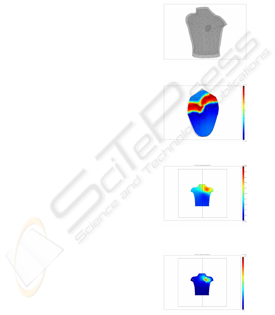
Figure 2 illustrates the activation wavefront in my-
ocardium at approximately t = 2T/3 after the acti-
vation where T is the time length of the heart cy-
cle. In Figure 3 we illustrate the body surface map of
the electric field (voltage) on the torso surface. Sim-
ilarly, Figure 4 illustrates the magnetic field map at
the same time. In Figure 5 we illustrate the mean
square error of the axis parameters with c = a/10
and b = a. The location of an anomaly was arbi-
trarily set to r
0
= (0,0.5,0.75). As expected, due
to the wavefront orientation as well as difference in
size, the estimation accuracy of the cross-sectional
axis parameters is much smaller. In Figure 6 we il-
lustrate the localization accuracy i.e., MSE of r
0
as a
function of noise. The SNR was defined as SNR =
10log(
∑
ky
lk
k
2
/σ
2
E
+ σ
2
B
).
6 CONCLUSIONS
We addressed the problem of localizing the diffusivity
disorder in the myocardium using ECG/MCG sensor
arrays. To model the cardiac activation we considered
an inhomogeneous reaction-diffusion model in a real
human torso. To model a the loss we used a paramet-
ric model for an oblate spheroid and set its conduc-
tivity to zero. We assumed that the remainder of the
myocardium tissue was homogeneous. The proposed
algorithm can be easily extended to account for an ar-
bitrary spatial variation in the diffusivity tensor using
a set of a priori known basis functions. In addition the
parametric shape of the anomaly can be extended to
model an arbitrary region using a three-dimensional
spatial Fourier transform. An effort should be made
to examine the sensitivity of the proposed algorithms
to the size of diffusivity difference between “regular”
tissue and anomaly as well as the number of the un-
known parameters needed to model arbitrary shapes.
Figure 1: Mesh geometry used for numerical study.
Figure 2: Activation wavefront, at t = 2T/3.
Figure 3: Body surface map of electric field at t = 2T/3.
Figure 4: Body surface map of magnetic field at t = 2T/3.
AN INVERSE MODEL FOR LOCALIZATION OF LOW-DIFFUSIVITY REGIONS IN THE HEART USING
ECG/MCG SENSOR ARRAYS
511

0 2 4 6 8 10 12 14
0.05
0.1
0.15
0.2
0.25
0.3
0.35
0.4
0.45
Size [cm]
MSE
Localization Mean Square Error − Size
MSE
a
MSE
c
Figure 5: Mean square error for estimating the size of the
anomaly.
1 3 5 7 9 11 13
0.02
0.04
0.06
0.08
0.10
0.12
0.14
0.16
0.18
0.2
0.22
SNR[dB]
MSE
Localization Mean Square Error − Position
Figure 6: Mean square error for estimating the location of
the anomaly.
REFERENCES
et al., L. Z. (2003). Heart-muscle fiber reconstruction from
diffusion tensor mri. In Proc. 14th IEEE Visualization
Conference. IEEE.
FitzHugh, R. A. (1961). Impulses and physiological states
in theoretical models of nerve membrane. Biophys. J.
Geselowtiz, D. (1970). On the magnetic field generated out-
side an inhomogeneous volume conductor by internal
current sources. IEEE Trans. Magn., 6:346–347.
Gulrajani, R. M. (1998). Bioelectricity and Biomagnetism.
John Wiley & Sons, New York.
Malmivuo, J. and Plonsey, R. (1995). Bioelectromagnetism.
Oxford University Press, New York.
Panfilov, A. and Holden, A. V. (1997). Computational Biol-
ogy of the Heart. John Wiley & Sons, Chichester, 1st
edition.
Rogers, J. M. and McCulloch, A. D. (1994). A collocation-
galerkin finite element model of cardiac action poten-
tial propagation. IEEE Transactions on Biomedical
Engineering, 41:743–757.
Sachse, F. B. (2004). Computational Cardiology. Springer,
Berlin.
Vonesh, F. and Chinchilli, V. M. (1997). Linear and Non-
linear Models for the Analysis of Repeated Measure-
ments. Marcel Dekker, New York.
BIOSIGNALS 2008 - International Conference on Bio-inspired Systems and Signal Processing
512