LEVEL SET BRIAN SEGMENTATION WITH AGENT CLUSTERING

FOR INITIALISATION

Fast Level Set Based MRI Tissue Segmentation with Termite-Like Agent Clustering

for Parameter Initialization

David Feltell and Li Bai

School of Computer Science & IT, Nottingham University, Triumph Rd, Nottingham, UK

Keywords:

Level Set, Multi Agent Clustering, Image Segmentation.

Abstract:

This paper presents a novel 3D brain segmentation method based on level sets and bio-inspired methodologies.

Level set segmentation methods, although highly promising, require manual selection of seed positions and

thereshold parameters, along with manual reinitialisation to a new level set surface for each candidate region.

Here, the use of swarm intelligent mechanisms is used to provide all the statistical data and sample points

required, allowing automatic initialisation of multiple level set solvers. This is shown by segmentation of

white matter, grey matter and cerebro-spinal ﬂuid in a simulated T1 MRI scan, followed by direct comparison

between a commercial level application - FMRIB’s FAST - and the ground truth anatomical model.

1 INTRODUCTION

The solution to initial value problems by level set

methods has transformed the study of evolving inter-

faces and, along with the surge in available processing

power, provides a unique and promising methodology

for three-dimensional image segmentation. However,

the initialization of surfaces and tuning of parameters

almost universally requires human intervention. By

using agent based clustering and segmentation algo-

rithms, we can hope to automate this process to a large

extent, thus no longer relying on expert knowledge or

requiring multiple tedious trials for an acceptable re-

sult.

The paper begins by reviewing the history of level

set methods, leading to the method currently used in

this work. Following this is a brief review of the

mechanisms of swarm intelligence, leading to previ-

ous attempts at data clustering and image segmenta-

tion using agent based principles. Next, the imple-

mentation details are given of the level set solver,

followed by the agent-based initialization algorithm.

Finally, preliminary results of the system are shown

along with a discussion of its merits and the project’s

future direction.

1.1 Level Set Method

Level set methods for image segmentation rely on an

evolving closed surface deﬁned by a moving inter-

face, the front, which expands from a point out into

the image, ﬁtting itself to the region it is released

within, and smoothing any noise. Among the advan-

tages of level set methods is the natural ability for

a single surface to seemingly split apart and merge

without losing its identity. To accomplish this we add

a further spatial dimension, φ, to our problem space,

then we can in effect have a single surface in (n+ 1)-

dimensional space, even though from observation of

n dimensions we see two or more spatially distinct

closed surfaces. This is the essence of the level set

method and allows for topological changes to be han-

dled naturally. This is easily visualised in the 2D case:

for example Figure 1, where two 2D surfaces are pro-

jected to a 3D volume, where it is shown they are

mathematically part of the same object. Numerically,

each point in space U includes a scalar φ that can vary

dynamically as time progresses, via a speed function

F. Functionally, by taking a slice at time t of all points

in U where φ = 0, we are taking the 0

level set of the

function φ.

If we initialise φ to the signed distance from an

initial closed surface, then we can visualise φ as the

height at a certain point, and all the points in space

with a height of 0 make up our surface. Thus, as well

as handling topological changes naturally, the level

set approach also has the advantage that the gradient

across the surface at any given point on the interface

can be found using ∇φ, meaning the local curvature

can be determined. A curvature term gives the signed

210

Feltell D. and Bai L. (2008).

LEVEL SET BRIAN SEGMENTATION WITH AGENT CLUSTERING FOR INITIALISATION - Fast Level Set Based MRI Tissue Segmentation with

Termite-Like Agent Clustering for Parameter Initialization.

In Proceedings of the First International Conference on Bio-inspired Systems and Signal Processing, pages 210-217

DOI: 10.5220/0001067702100217

 SciTePress

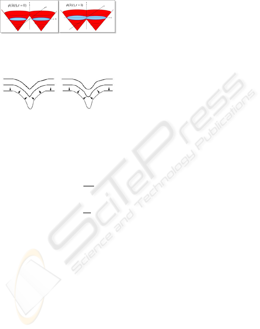
Figure 1: Illustration of level set function surface S (red)

and evolution of moving interface/zero level set (blue).

Topological change of two separate fronts (left) into a sin-

gle front (right) handled naturally via higher dimensional

function. After (Sethian, 1996).

Figure 2: Illustration of surface evolution without curva-

ture (left) and using a curvature term (right). After (Sethian,

1996).

’sharpness’ of the interface at a point, allowing for

a smoothing effect, overcoming noise and preventing

leaks. This is illustrated in Figure 2. The typical for-

mulation for the φ update function then becomes:

= |∇φ|(αF + (1− α)∇•

∇φ

|∇φ|

) (1)

Where: φ

is the time derivative of φ; α controls

the the level of smoothness in the surface; F is the

data-dependent speed function; ∇ •

∇φ

|∇φ|

gives local

curvature at a given point.

Updating the values of φ at each point in space

requires a numerical technique to evolve the zero

level set from an initial speciﬁcation. Naively then,

we could initialise a surface in space, create a suit-

able speed function F, and numerically integrate until

some condition is met and the surface extracted as all

points where φ = 0 (for example (Phillips, 1999)). An

advantage here is sub-cell accuracy - the φ values can

be interpolated to ﬁnd points on a scale that is more

accurate than the discrete embedding it is operating

within. The ﬁrst problem here is that the whole state-

space must be evaluated each iteration, rather than

just the surface. Secondly a small timestep is required

to prevent numerical instabilities. These two caveats

make the naive method undesirable for use outside of

specialist ﬁelds.

Algorithms have been developed to overcome

these issues by only performing updates on regions

near the surface, rather than integrating over the entire

state space. The most well-knownis the Narrow Band

approach (D. Adalsteinsson, 1995; Sethian, 1999),

where numerical integration is performed within a

band of points initialised around the surface, though

when the zero level set reaches the edge of this band,

the band must be reset. This dramatically increases

efﬁciency over the naive method, with little or no ef-

fect on accuracy. However, further optimization in

this vein has come in the form of the Sparse Field ap-

proach (Whitaker, 1998). With this method the nar-

row band is reduced to the smallest workable size and

the reinitialisation requirement is based on a purely

local update, rather than a global update of the entire

band. The reduction in accuracy is tolerable for most

applications and its implementation has allowed the

level set family of methods to achieve real-time per-

formance levels in complex 3D applications (for ex-

ample see (Lefohn et al., 2003; Lefohn et al., 2004)).

The Sparse Field approach has been taken even

further in the work of (Karl, 2005), and is the method

presented here. In this work the narrow band is low-

ered to simply two linked lists operating in a discrete

space, L

and L

out

, representing the inside and out-

side boundaries of the zero level set, respectively. No

attempt at sub-cell accuracy is made and most op-

erations use integer math. The values of φ are also

kept constant depending on their status and are up-

dated discretely. There are four such values repre-

senting inside, inside edge, outside edge, and outside

the volume, set so that a rough gradient can be found

at any point (for example: 3,1,−1,−3, respectively).

The level set algorithm approximation itself is imple-

mented in a two-pass process:

In the ﬁrst pass elements in L

and L

out

are

checked using the speed function F. If an expan-

sion/contraction is provoked, the relevant list element

is switched to the opposing list. If an element ﬁnds

itself surrounded by cells with φ values of opposite

sign, it is removed from its list. This fact allows for

splits and merges in the topology.

The second phase involves an approximate Gaus-

sian smoothing term G, that is, taking the (weighted)

average of φ values from the area surrounding an el-

ement of L

or L

out

. Depending on the outcome of

G, expansion/contraction adjustments to the lists and

φ values are performed, similar to expansion via F.

This has the effect of smoothing away noise as well

as sharp protuberances in the surface.

Unlike previous algorithms, the process of expan-

sion via the speed function and contraction via curva-

ture are not intrinsically linked into the same update.

In this algorithm, F is run on L

and L

out

a number of

times. After this initial expansion phase a number of

G runs are similarly done on L

and L

out

. The ratio of

F to G runs determines the smoothness of the solution

(in an analogue to the α parameter in (1)).

LEVEL SET BRAIN SEGMENTATION WITH AGENT CLUSTERING FOR INITIALISATION - Fast Level Set Based

MRI Tissue Segmentation with Termite-Like Agent Clustering for Parameter Initialization

211

Further optimization can be made when the ratio

of F runs is much higher than G runs. Elements vis-

ited on the list that have reached a locally optimal po-

sition will remain in that position on the next run of

the speed function. Therefore they can be removed

from successive F runs on that pass.

As mentioned in their paper title, this method de-

parts almost entirely from the PDE based methods,

but maintains many of the advantages. Sub cell accu-

racy is not possible in this generic form, but it would

a simple addition to use this method as a prototype

generator for slower, but more accurate methods. The

inclusion of the φ embedding, albeit much simpliﬁed,

allows local topology to be determined at any point

to discrete-level accuracy. Thus, the Gaussian func-

tion has the information required to approximate the

’sharpness’ at a point, and to expand or contract as a

result (in a reasonable approximation to the effect of

curvature). The lack of the requirement to solve PDEs

holds several advantages. No timestep is required in

the update process - the algorithm is entirely discrete.

The method maintains the implicit ability of splits and

merges along the front, without relying on any gra-

dient calculation, eliminating the need for expensive

entropy-satisfying spatial derivative schemes.

Parameter selection for level set segmentation

generally requires at least some level of human in-

teraction. Speciﬁcally in the case of image segmen-

tation, initialization of a level set solver requires at

minimum seed locations, an ideal data value, and an

acceptable noise threshold to be preset. Also, differ-

ing data classes in the same problem space, for exam-

ple tissue types in medical scans, each require their

own level set surface with their own set of initializa-

tion parameters. Ideally the task of assigning seed

locations and calculating level set parameters would

be automated. These issues lend themselves well to

an agent based approach, which will be discussed in

the following section.

1.2 Multi-Agent Swarm Based

Algorithms

Agents are independent entities existing in some

environment - sensing, processing and modifying

the environment based on internal reasoning. For

multi-agent systems, the swarm intelligence and self-

organisation paradigms have become popularized in

many disciplines as an explanation for the apparent

mismatch in complexity of agent versus complexity

of task (Camazine et al., 2001), and as a unique engi-

neering metaphor (Bonabeau et al., 1999). Such sys-

tems of agents can focus on simple stimulus-response

functions using purely local stimuli with little or no

cognition or direct communication. Tasks are ac-

complished by exploiting the non-linearity inherent

in such a massively parallel system, rather than re-

lying on individual agent complexity. An agent mod-

ifying the environment at a particular location allows

another agent in that same location at a later time

to sense this new state and respond accordingly. In

this way the environment is used for indirect com-

munication, termed stigmergy. Stigmergy in bio-

logical systems is further enhanced by the complex-

ity of the environment, for example diffusion is uti-

lized in many biological processes to spread infor-

mation in the form of chemical gradients. Activa-

tion/attraction and inhibition/repulsion functions can

thus be designed to control agent interactions based

solely on local environmental state and any internal

state, relying on quantitative information reinforce-

ment and decay as well as qualitative signaling via the

environment to control the weighting between possi-

ble responses. A global-level task or structure may

then be many times more complex than an individual

can perceive or accomplish, yet through parallel ap-

plication of simple rules with indirect non-linear cou-

plings, we see the spontaneous emergence of a solu-

tion. Given this non-linearity, a tiny change in a pa-

rameter can result in a drastically different solution,

but (if the system is well formed) one that still con-

forms to a valid set of stable solutions - that is, the

system exhibits multistability. We have demonstrated

this engineering paradigm previously in modeling the

building behaviour of Macrotermes termites (Feltell

and Bai, 2004; Feltell et al., 2005). The use of an

attractive cement pheromone to coordinate soil clus-

tering behaviour has provided the inspiration for the

swarm-intelligent clustering mechanism used here.

Swarm based clustering algorithms have been de-

veloped to cluster sets of n-dimensional data, gen-

erally projected onto a 2D grid, by taking inspira-

tion from brood sorting and corpse clustering in ants

(Monmarche et al., 1999; Monmarche, 1999; Kanade

and Hall, 2003; Schockaert et al., 2004) as well as

building behaviour in termites (Vizine et al., 2005).

The approach does not need any prior knowledge of

the problem space or number of clusters, and as a

bonus gives a visual representation of the clusters on

the 2D grid.

Agent based approaches have also been devel-

oped to directly segment an image, again using in-

spiration from natural systems such as ant pheromone

trail networks (Ramos and Almeida, 2000), artiﬁcial

life (Liu et al., 1997; Liu and Tang, 1999; Bocchi

et al., 2005), social spiders (Bourjot et al., 2003), and

even termites, bloodhounds and children (Fledelius

and Mayoh, 2006). Here the agents interact directly

BIOSIGNALS 2008 - International Conference on Bio-inspired Systems and Signal Processing

212

within the n-dimensions of the problem space, rather

than outside it. This distinction from swarm based

data clustering allows spatially localized regions to be

processed independently - possibly requiring only a

subset of the image space to be explored.

If the two perspectives can be combined, along

with other swarm-inspired mechanisms, we could

ideally form a localized data clustering algorithm,

whereby ideal seed locations and other parameters

would be found by agents within the image environ-

ment as they cluster similar voxels together.

Swarm intelligent systems emphasize robustness

and diversity over accuracy, and so ﬁnd solutions to

complex problems that are ’good enough’, but which

require minimal agent capability in terms of both cog-

nition and interaction. One of the major lures of level

set algorithms is the tolerance for error, both in the

problem space and, within limits, the initialization

parameters. As long as ’good enough’ seed loca-

tion, ideal value and acceptable range parameters can

be determined, the solution to the level set equations

should be near-optimal in all but the hardest cases.

With this assumption in mind, well located seeds can

then be acceptable sample points used to approximate

the voxel mean and range within a class.

2 IMPLEMENTATION

2.1 Level Set Solver

The level set solver is derived from the model of Shi

& Karl (Karl, 2005). We deﬁne two sets of discretized

points, representing the inside and outside layers be-

tween which lies the level set surface. As well as up-

dating these sets as the surface expands or contracts

we must maintain the values of φ, such that φ = 3

inside the volume enclosed by the level set surface,

φ = 1 along the inside layer, φ = −1 along the outside

layer, and φ = −3 outside the volume (note: the sign

is reversed here compared to the original algorithm to

be more in line with other level set methodologies).

Finally, we must ensure that no orphaned points exist.

That is, inside points must always have at least one

outside point adjacent to them, and similarly outside

points must always have at least one inside point ad-

jacent. The update routine for both inside and outside

layers is similar, though varies in parameter value.

Following is a summary of the general update routine:

Let:

• Current time step be t.

• Two sets of points deﬁning our two discretized

layers be S

and S

• φ constants in space be: b

along S

; b

along S

; a

in the volume beyond S

; a

in the volume beyond

• Three-dimensional cartesian point vector, p =

(pi+ p j + pk).

• Neighbourhood of p, N(p) = {(pi + i + pj +

pk),(pi − i + pj + pk),(pi + pj + j + pk),(pi +

pj − j + pk), (pi + p j + pk + k),(pi+ pj + pk −

k)}.

• Context dependent speed function, F(p) : ℜ −→

ℜ, with condition f

required for update to occur.

Here and throughout this work it is assumed voxel

intensity value is in [0,1] ∈ ℜ.

Then, for each p ∈ S

, iff F(p) =⇒ f

1. Increment time step, t.

t ←− t + 1 (2)

2. p is added to S

←− {S

∪ {p}} (3)

3. φ at point p is set to constant, b

φ(p,t) ←− b

(4)

4. p is removed from S

, whilst all relevant neigh-

bours of p are added to S

←− {S

− {p}} ∪ {∀r ∈ N(p) | φ(r,t) = a

}

(5)

5. φ at all relevant neighbours of point p is set to

constant, b

φ({r | φ(r,t) = a

},t) ←− b

,∀r ∈ N(p) (6)

6. All points in S

that are in not neighboured by a

point in S

are orphaned points and must be re-

moved.

←− S

− {∀r ∈ S

| N(r) ∩ S

0} (7)

7. φ at all orphaned points in S

is set to constant, a

φ({r | N(r) ∩ S

0},t) ←− a

,∀r ∈ S

(8)

In practice, all these steps can be combined into a sin-

gle update loop. The update loop is performedon both

the inside and outside layers. Let our inside surface

be S

and the outside surface be S

out

, then: a

= 3,

out

= −3, b

= 1, b

out

= −1, f

⇔ (F(p) > 0),

out

⇔ (F(p) < 0). The steps (3)..(6) deal with the

surface evolution. The steps (7) and (8) handle shock

propagation, that is, they remove points as the curve

crosses over itself to maintain an unambiguous closed

surface.

LEVEL SET BRAIN SEGMENTATION WITH AGENT CLUSTERING FOR INITIALISATION - Fast Level Set Based

MRI Tissue Segmentation with Termite-Like Agent Clustering for Parameter Initialization

213

The algorithm is then:

Let:

• D(p) be the problem speciﬁc data term, speciﬁ-

cally the voxel gray level value at point p.

• J(p) be the problem speciﬁc speed function,

speciﬁcally: J(p) = 1 for |(D(p) − T)| < ε and

J(p) = −1 for |(D(p) − T)| > ε, where: T is the

ideal data value; ε is the acceptable error.

• G(p) be a Gaussian smoothing approximation,

speciﬁcally G(p) =



φ(p,t) +

∑

r∈N(p)

φ(r,t)



/7.

With the condition G(p) = 0 iff |G(p)| < 1, tighter

areas can be explored, as smoother curves will

neither contract nor expand. This produces more

accurate solutions in most cases, but tends to give

less smooth surfaces.

• t

be the number of speed runs to perform; t

the number of Gaussian smoothing runs to per-

form.

Then:

A Initialize S

and S

out

to small surface(s) about

given seed locations.

B Perform (2)..(8) with: i = out; j = in; F(p) =

J(p).

C Perform (2)..(8) with i= in; j = out; F(p) = J(p).

D Repeat from (B) while t < t

E Perform (2)..(8) with: i = out; j = in; F(p) =

G(p).

F Perform (2)..(8) with i = in; j = out; F(p) =

G(p).

G Repeat from (E) while t < t

+ t

H Set t = 0. Repeat from (B) for t

iterations.

2.2 Swarm based Parameter

Initialization

The parameter speciﬁcation for the level set solver as

well as the number of tissue typesrequiring individual

segmentation is beyond the capability of a level set al-

gorithm alone. Instead, in this work we show how we

can use a collection of agents following similar rules

to previous agent clustering algorithms, but with the

agents embodied within the image space itself, ﬁnd-

ing good seed locations as well as performing minor

preprocessing functions.

Agents have real-valued position and direction,

using simple nearest neighbour approximation when

sensing the underlying discrete image voxels. They

wander the image in an initially random direction,

however as they move they lay a quantity of attrac-

tive ’pheromone’ in visited voxels. The quantity of

pheromone is proportional to the divergence of voxel

intensity |∇

· D| at their current location. A high di-

vergence value often indicates a heterogeneity in the

image - speciﬁcally an interface between two regions.

Here, pheromone deposition further has the restric-

tion D > 0.1 to avoid segmenting irrelevant black re-

gions. Pheromone diffuses through the image lattice,

with the edge of the lattice and near-black (D < 0.1)

voxels acting as sinks. The addition of a positive re-

inforcement pheromone mechanism allows the agents

to use gradient following behaviour in coordinating

toward promising seed locations. As pheromone dif-

fuses away it causes that area to receive less attention,

ultimately meaning less suitable seed locations are

abandoned. This reﬂects in many ways the clustering

behaviour of termites in nest construction (Bruinsma,

1979), where heterogeneities stimulate deposits of

soil laden with a cement pheromone, which in turn

attracts other termite builders to the site.

This clustering behaviour, in the termite case, cre-

ates regular spaced piles or pillars of soil. Piles close

to one-another thus compete for the termites atten-

tions, eventually resulting in regularly spaced pillars.

In this work, as with the termite paradigm, this mech-

anism means seed locations tend not to become too

localised. The combined effect ultimately increases

the agents’ sampling efﬁciency within large images.

The generalised update routine for an individual

agent is given as follows:

Let:

• t be the current time step of an agent.

• Real-valued point vector, p be the current position

of an agent

• Scalar pheromone ﬁeld, ρ(p) be the pheromone

concentration at location p.

• Speed, s be a scalar speed value for the agent.

• Vector v be the continuous direction vector of the

agent.

Then:

1. Increment time step, t.

t ←− t + 1 (9)

2. Lay pheromone proportional to the logarithm of

the absolute divergence. Logarithmicscale is used

here to avoid ﬂoating point accuracy overﬂow.

log(ρ(p)) ←− log



ρ(p) + |∇

D(p)|



(10)

3. Calculate new direction vector from weighted gra-

dient of logρ.

v ←− v+ α(v− ∇logρ) (11)

BIOSIGNALS 2008 - International Conference on Bio-inspired Systems and Signal Processing

214

4. Calculate speed scalar based on local density of ρ.

s ←− 1+

1+ log(ρ(p))

(12)

5. Calculate updated position based on normalized

direction vector and speed value.

p ←− p+

||v||

· s (13)

Where: α is the weighting of pheromonegradients

in movement; β controls the maximum speed of an

agent.

The full agent algorithm is then:

A Initialize set of n agents, M, each with random

position within the image and random direction.

B Perform (9)..(13) for each m ∈ M.

C Diffuse pheromone: ∂

ρ = d · ∇

D Repeat from (B) while t < t

time steps.

E Select the top C voxel locations with highest

pheromone level ρ, to get full seed list, Q.

F Run k-means clustering on Q, classifying into

prespeciﬁed number of sets, Q

, where i =

{1,2,..,q}.

G Within each Q

calculate mean µ(Q

) and standard

deviation σ(Q

), givingideal data value T = µ(Q

)

and error threshold ε = σ(Q

) + k, where k is a

constant, within a class.

Once T and ε have been calculated for a seed set

, the level set routine can be run, initialising L

and L

out

surfaces as pseudo-spheres about each seed

location in Q

. The agent algorithm need only be run

once, then the level set algorithm run once for each

seed set.

Additionally, in practice the diffusion step can

be moved into a separate thread to take advantage

of modern day multiple core processors. With the

simplest distributed setup, with little control on syn-

chronization or load balancing, the algorithm can still

function correctly - an implicit advantage of the ro-

bust swarm metaphor.

The image is ﬁnally extracted as all voxel posi-

tions where φ > 0, thus all points lying on and within

3 RESULTS

The dataset used comes from BrainWeb’s online MRI

simulator (McConnell BIC, 2007) with default pa-

rameters: modality T1, slice thickness 1mm, noise

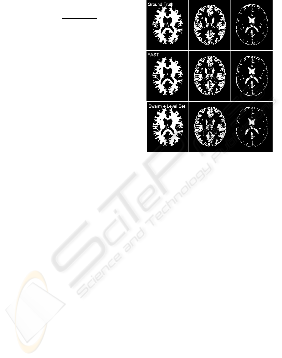
Figure 3: Comparison of ground truth to FAST and the

swarm initialised level set solution presented here. Images

used in both FAST and the present work have been prepro-

cessed by BET. From left to right: white matter; gray mat-

ter; cerebro-spinal ﬂuid.

3% and non-uniform intensity 20%. For comparison

with ground truth and FAST (Zhang et al., 2001) the

number of classes is set q = 3. The various parame-

ters, unless otherwise stated, are set as follows:

α = 2;β = 2.5;d = 0.015;k = 0.02;t

= 10;t

3000;t

= 30;t

= 3

The parameter values above for α,β,d and k, were

found in part using a real-valued genetic algorithm,

using the similarity to the ground truth images, mi-

nus the similarity between one another, as a ﬁtness

function. This process has proven useful so far, yet

is only partially utilised here and remains a direction

for future work. Other values are chosen intuitively to

balance execution time and accuracy.

From Figure 3 it can be seen how the approach,

even in this early stage, can compete with popular so-

lutions such as FMRIB’s FAST, which uses a method

based on Markov random ﬁelds. In both solutions,

preprocessing has been performed using FMRIB’s

popular BET (Smith, 2002) to skull strip and nor-

malise the image voxels.

Quantitative measurement on accuracy is approx-

imately possible given the hand segmented ground

truth images available. In the above case, FAST

achieves approximately 92%, 85% and 57% accu-

racy, whereas the swarm initialised level set algorithm

LEVEL SET BRAIN SEGMENTATION WITH AGENT CLUSTERING FOR INITIALISATION - Fast Level Set Based

MRI Tissue Segmentation with Termite-Like Agent Clustering for Parameter Initialization

215

achieves 86%, 83% and 55%, for white matter, grey

matter and cerebro spinal ﬂuid, respectively. FAST

remains superior, but the small score difference cer-

tainly indicates the presented approach is well worth

further investigation.

In terms of execution time, from the point of ﬁle

loading to ﬁnal ﬁle output, FAST outdoes the perfor-

mance of the presented work by just over double. The

above solution was found by the swarm initialised

level set algorithm in approximately 17 mins, whereas

FAST ﬁnished in approximately 8 mins. It is worth

noting that the swarm approach presented is still in

early development, and as discussed in the next sec-

tion, has the advantage of naturally supporting a dis-

tributed implementation.

4 DISCUSSION AND FUTURE

WORK

The level set solver is an approximate discrete solu-

tion to a continuous problem. Although the algorithm

used in this work is particularly fast, it simply does

not have the power of a narrow band or even sparse

ﬁeld approach. These methods not only reﬂect the

naive approach more directly, but also have sub-cell

accuracy, where actual surface points can be interpo-

lated within image voxels using the real-valued gradi-

ent of φ. They can also vary in speed along different

areas of the surface, allowing for a more global curva-

ture force effect. The discretisation of φ values to sim-

ply the set {−3,−1, 1, 3} means the curvature term is

much more rigid, and does not distinguish on a lo-

cal level between corners of differing sharpness. Ide-

ally the current level set solver approximation would

work as a rapid prototype for a more accurate narrow

band based method. This remains a direction for fu-

ture work.

One beneﬁt of using a swarm based system is in

the robustness to a noisy environment. In this regard

it should be possible to include an atlas mechanism,

using only the most minimal registration with the can-

didate image, and restrict agent interaction within or

near the atlas template for a given region. This would

give the agents’ environment a signiﬁcant amount of

extra information, which can be used to focus agent

efforts - increasing efﬁciency and allowing for seg-

mentation of more difﬁcult (too smooth/too noisy) re-

gions.

The preprocessing by BET could be removed for

future versions. BET simpliﬁes segmentation signif-

icantly, and prevents areas such as the skull being

segmented as part of brain matter. However, pre-

liminary results of segmentation without BET pre-

Figure 4: Solution found using current algorithm without

BET preprocessing. All parameters are set similar - the

number of classes remaining at 3. From left to right: white

matter, gray matter, cerebro-spinal ﬂuid.

processing are promising in their own right, though

show several mismatched regions (see Figure 4), and

it is likely that with more classes and ground truth

samples, along with evolutionary algorithm parameter

tuning, the method can be applied to multiple modal-

ities and varying image spaces without the need for

any preprocessing.

Another beneﬁt of the multi-agent paradigm is its

naturally distributed nature. As has been eluded to,

the diffusion of pheromone can already be ported to

another processing unit to greatly increase efﬁciency.

A further extension could see the image space and/or

agents split to run parallel. Certainly each region’s

level set solver could in future run on separate pro-

cesses to dramatically decrease execution time.

REFERENCES

Bocchi, L., Ballerini, L., and Hssler, S. (2005). A new evo-

lutionary algorithm for image segmentation. Applica-

tions on Evolutionary Computing, pages 264–273.

Bonabeau, E., Dorigo, M., and Theraulaz, G. (1999).

Swarm Intelligence: From Natural to Artiﬁcial Sys-

tems. Oxford University Press.

Bourjot, C., Chevrier, V., and Thomas, V. (2003). A new

swarm mechanism based on social spiders colonies:

From web weaving to region detection. Web Intelli-

gence and Agent System, 1(1):13–32.

Bruinsma, O. (1979). An Analysis of Building Behaviour of

the Termite Macrotermes Subhyalinus (Rambur). PhD

thesis, Landbouwhogeschool, Wageningen.

Camazine, S., Deneubourg, J.-L., Franks, N., Sneyd, J.,

Theraulaz, G., and Bonabeau, E. (2001). Self-

Organization in Biological Systems. Princeton Uni-

versity Press.

D. Adalsteinsson, J. S. (1995). A fast level set method for

propagating interfaces. J. Comp. Phys., 118:269–277.

Feltell, D. and Bai, L. (2004). Swarm robotics for con-

struction. In 24th SGAI International Conference on

Innovative Techniques and Applications of Artiﬁcial

Intelligence, Cambridge, UK.

BIOSIGNALS 2008 - International Conference on Bio-inspired Systems and Signal Processing

216

Feltell, D., Bai, L., and Soar, R. (2005). Bio-inspired emer-

gent construction. In IEEE 2nd Intl. Swarm Intelli-

gence Symposium, Pasadena, CA, USA.

Fledelius, W. and Mayoh, B. (2006). A swarm based ap-

proach to medical image analysis. In 24th IASTED In-

ternational Conference on Artiﬁcial Intelligence and

Applications (AIA 2006), pages 150–155, Anaheim,

CA, USA. ACTA Press.

Kanade, P. and Hall, L. (2003). Fuzzy ants as a cluster-

ing concept. In 22nd International Conference of the

North American Fuzzy Information Processing Soci-

ety (NAFIPS), pages 227–232.

Karl, Y. S. W. (2005). A fast level set method without solv-

ing pdes. In IEEE International Conference on Acous-

tics, Speech, and Signal Processing (ICASSP 2005),

volume 2, pages 97–100.

Lefohn, A. E., Cates, J. E., and Whitaker, R. T. (2003). In-

teractive, gpu-based level sets for 3d segmentation. In

Medical Image Computing and Computer-Assisted In-

tervention (MICCAI 2003), pages 564–572.

Lefohn, A. E., Kniss, J. M., Hansen, C. D., and Whitaker,

R. T. (2004). A streaming narrow-band algorithm: In-

teractive computation and visualization of level sets.

IEEE Transactions on Visualization and Computer

Graphics, 10:422–433.

Liu, J. and Tang, Y. (1999). Adaptive image segmentation

with distributed behavior-based agents. IEEE Trans-

actions on Pattern Analysis and Machine Intelligence,

21:544–551.

Liu, J., Tang, Y., and Cao, Y. (1997). An evolutionary

autonomous agents approach to image feature extrac-

tion. IEEE Transactions on Evolutionary Computa-

tion, 1:141–158.

McConnell BIC (2007). Brainweb: Simulated

brain database, Montreal Neurological Institute.

http://www.bic.mni.mcgill.ca/brainweb/.

Monmarche, N. (1999). On data clustering with artiﬁcial

ants. In Freitas, A. A., editor, Data Mining with Evo-

lutionary Algorithms: Research Directions, pages 23–

26, Orlando, Florida. AAAI Press.

Monmarche, N., Slimane, M., and Venturini, G. (1999). On

improving clustering in numerical databases with arti-

ﬁcial ants. In ECAL ’99: Proceedings of the 5th Euro-

pean Conference on Advances in Artiﬁcial Life, pages

626–635, London, UK. Springer-Verlag.

Phillips, C. L. (1999). The level set method. The MIT Un-

dergraduate Journal of Mathematics, 1:155–164.

Ramos, V. and Almeida, F. (2000). Artiﬁcial ant colonies in

digital image habitats - a mass behaviour effect study

on pattern recognition. In 2nd Int. Workshop on Ant

Algorithms (ANTS 2000), pages 113–116, Brussels,

Belgium.

Schockaert, S., Cock, M. D., Cornelis, C., and Kerre, E. E.

(2004). Fuzzy ant based clustering. In International

Workshop on Ant Colony Optimization and Swarm

Intelligence (ANTS 2004), pages 342–349, Brussels,

Belguim.

Sethian, J. (1996). Level set methods: An act of vio-

lence - evolving interfaces in geometry, ﬂuid mechan-

ics, computer vision and materials sciences. American

Scientist.

Sethian, J. (1999). Level Set Methods and Fast Marching

Methods. Cambridge University Press.

Smith, S. (2002). Fast robust automated brain extraction.

Human Brain Mapping, 17(3):143–155.

Vizine, A., de Castro, L., Hruschka, E., and Gudwin, R.

(2005). Towards improving clustering ants: An adap-

tive ant clustering algorithm. Informatica, 29(2):143–

154.

Whitaker, R. (1998). A level-set approach to 3d reconstruc-

tion from range data. International Journal of Com-

puter Vision, 29(3):203–231.

Zhang, Y., Brady, M., and Smith, S. (2001). Segmentation

of brain mr images through a hidden markov random

ﬁeld model and the expectation maximization algo-

rithm. IEEE Trans. on Medical Imaging, 20(1):45–57.

LEVEL SET BRAIN SEGMENTATION WITH AGENT CLUSTERING FOR INITIALISATION - Fast Level Set Based

MRI Tissue Segmentation with Termite-Like Agent Clustering for Parameter Initialization

217