NOISE REDUCTION AND VOICE SEPARATION ALGORITHMS

APPLIED TO WOLF POPULATION COUNTING

B. Dugnol, C. Fern´andez, G. Galiano and J. Velasco

Dpto. de Matemticas, Universidad de Oviedo, c/ Calvo Sotelo s/n, 33007 Oviedo, Spain

Keywords:

Time-frequency distribution, instantaneous frequency, signal separation, noise reduction, chirplet transform,

partial differential equation, population counting.

Abstract:

We use signal and image theory based algorithms to produce estimations of the number of wolves emitting

howls or barks in a given ﬁeld recording as an individuals counting alternative to the traditional trace collecting

methodologies. We proceed in two steps. Firstly, we clean and enhance the signal by using PDE based image

processing algorithms applied to the signal spectrogram. Secondly, assuming that the wolves chorus may be

modelled as an addition of nonlinear chirps, we use the quadratic energy distribution corresponding to the

Chirplet Transform of the signal to produce estimates of the corresponding instantaneous frequencies, chirp-

rates and amplitudes at each instant of the recording. We ﬁnally establish suitable criteria to decide how such

estimates are connected in time.

1 INTRODUCTION

Wolf is a protected specie in many countries around

the world. Due to their predator character and to

their proximity to human settlements, wolves often

kill cattle interfering in this way in farmers’ econ-

omy. To smooth this interference, authorities reim-

burse the cost of these lost to farmers. Counting the

population of wolves inhabiting a region is, therefore,

not only a question of biological interest but also of

economic interest, since authorities are willing to es-

timate the budget devoted to costs produced by wolf

protection, see for instance (Skonhoft, 2006). How-

ever, estimating the population of wild species is not

an easy task. In particular, for mammals, few and not

very precise techniques are used, mainly based on the

recuperation of ﬁeld traces, such as steps, excrements

and so on. Our investigation is centered in what it

seems to be a new technique, based on signal and

image theory methods, to estimate the population of

species which fulﬁll two conditions: living in groups,

for instance, packs of wolves,and emitting some char-

acteristic sounds, howls and barks, for wolves. The

basic initial idea is to produce, from a given record-

ing, some time-frequencydistribution which allows to

identify the different howls corresponding to different

individuals by estimating the instantaneous frequency

(IF) lines of their howls.

Unfortunately, the real situation is somehow more

involved due mainly to the following two factors. On

one hand, since natural sounds, in particular wolf

howling, are composed by a fundamental pitch and

several harmonics, direct instantaneous frequency es-

timation of the multi-signal recording leads to an

over-counting of individuals since various IF lines

correspond to the same individual. Therefore, more

sophisticated methods are indicated for the analysis

of these signals, methods capable of extracting addi-

tional information such as the slope of the IF, which

allows to a better identiﬁcation of the harmonics of a

given fundamental tone. The use of a Chirplet type

transform (S. Mann, 1995; L. Angrisani, 2002) is in-

vestigated in this article, although an equivalent for-

mulation in terms of the Fourier fractional transform

(H. M. Ozaktas, 2001) could be employed as well.

On the other hand, despite the quality of recording

devices, ﬁeld recordings are affected for a variety of

undesirable signals which range from low amplitude

broad spectrum long duration signals, like wind, to

signals localized in time, like cattle bells, or localized

Dugnol B., Fernández C., Galiano G. and Velasco J. (2008).

NOISE REDUCTION AND VOICE SEPARATION ALGORITHMS APPLIED TO WOLF POPULATION COUNTING.

In Proceedings of the First International Conference on Bio-inspired Systems and Signal Processing, pages 77-84

DOI: 10.5220/0001057000770084

 SciTePress

in spectrum, like car engines. Clearly, the addition

of all these signals generates an unstructured noise

in the background of the wolves chorus which im-

pedes the above mentioned methods to work properly,

and which should be treated in advance. We accom-

plish this task by using PDE-based techniques which

transforms the image of the signal spectrogram into

a smoothed and enhanced approximation to the reas-

signed spectrogram introduced in (K. Kodera, 1978;

F. Auger, 1995) as a spectrogram readability improv-

ing method.

2 SIGNAL ENHANCEMENT

In previous works (B. Dugnol, 2007a; B. Dugnol,

2007d), we investigated the noise reduction and edge

(IF lines) enhancement on the spectrogram image by a

PDE-based image processing algorithm. For a clean

signal, the method allows to produce an approxima-

tion to the reassigned spectrogram through a pro-

cess referred to as differential reassignment, and for a

noisy signal this process is modiﬁed by the introduc-

tion of a nonlinear operator which induces isotropic

diffusion (noise smoothing) in regions with low gra-

dient values, and anisotropic diffusion (edge-IF en-

hancement) in regions with high gradient values.

Let x ∈ L

(R) denote an audio signal and consider

the Short Time Fourier transform (STFT)

(x;t,ω) =

x(s)ϕ(s− t)e

−iωs

ds, (1)

corresponding to the real, symmetric and normalized

window ϕ ∈ L

(R). The energy density function or

spectrogram of x corresponding to the window ϕ is

given by

(x;t,ω) = |G

(x;t,ω)|

, (2)

which may be expressed also as (Mallat, 1998)

(x;t,ω) =

WV(ϕ;

ω)WV(x;t−

t,ω−

ω)d

ω,

(3)

with WV(y;·,·) denoting the Wigner-Ville distribu-

tion of y ∈ L

(R),

WV(y;t,ω) =

y(t +

)y(t −

−iws

ds.

The Wigner-Ville (WV) distribution has received

much attention for IF estimation due to its excel-

lent concentration and many other desirable math-

ematical properties, see (Mallat, 1998). However,

it is well known that it presents high amplitude

sign-varying cross-terms for multi-component signals

which makes its interpretation difﬁcult. Expression

(3) represents the spectrogram as the convolution of

the WV distribution of the signal, x, with the smooth-

ing kernel deﬁned by the WV distribution of the

window, ϕ, explaining the mechanism of attenuation

of the cross-terms interferences in the spectrogram.

However, an important drawback of the spectrogram

with respect to the WV distribution is the broadening

of the IF lines as a direct consequence of the smooth-

ing convolution. To override this inconvenient, it was

suggested in (K. Kodera, 1978) that instead of assign-

ing the averaged energy to the geometric center of the

smoothing kernel, (t,ω), as it is done for the spectro-

gram, one assigns it to the center of gravity of these

energy contributions, (

ω), which is certainly more

representative of the local energy distribution of the

signal. As deduced in (F. Auger, 1995), the gravity

center may be computed by the following formulas

t(x;t,ω) = t − ℜ



Tϕ

(x;t,ω)



ω(x;t,ω) = ω + ℑ



Dϕ

(x;t,ω)



where the STFT’s windows in the numerators are

Tϕ(t) = tϕ(t) and Dϕ(t) = ϕ

′

(t). The reassigned

spectrogram, RS

(x;t,ω), is then deﬁned as the ag-

gregation of the reassigned energies to their cor-

responding locations in the time-frequency domain.

Observe that energy is conserved through the reas-

signment process. Other desirable properties, among

which non-negativity and perfect localization of lin-

ear chirps, are proven in (Auger, 1991). For our ap-

plication, it is of special interest the fact that the re-

allocation vector, r(t,ω) = (

t(t,ω) − t,

ω(t,ω) − ω),

may be expressed through a potential related to the

spectrogram (E. Chassandre-Mottin, 1997),

r(t,ω) =

∇log(S

(x;t,ω)), (4)

when ϕ is a Gaussian window of unit variance. Let

τ ≥ 0 denote an artiﬁcial time and consider the dy-

namical expression of the reassignment given by

Φ(t,ω,τ) = (t,ω)+τr(t,ω) which, for τ = 0 to τ = 1,

connects the initial point (t,ω) with its reassigned

point (

ω). Rewriting this expression as

(Φ(t, ω,τ) − Φ(0,ω,τ)) = r(t,ω),

and taking the limit τ → 0, we may identify the dis-

placement vector r as the velocity ﬁeld of the trans-

formation Φ. In close relation with this approach

is the process referred to as differential reassignment

(E. Chassandre-Mottin, 1997), deﬁned as the transfor-

mation given by the dynamical system corresponding

BIOSIGNALS 2008 - International Conference on Bio-inspired Systems and Signal Processing

to such velocity ﬁeld,

(

dχ

dτ

(t,ω,τ) = r(χ(t,ω,τ)),

χ(t, ω,0) = (t,ω),

(5)

for τ > 0. Observe that, in a ﬁrst order approximation,

we still have that χ connects (t,ω) with some point in

a neighborhood of (

ω), since

χ(t, ω,1) ≈ χ(t,ω, 0) + r(χ(t,ω,0))

= (t,ω) + r(t,ω) = (

ω).

In addition, for τ → ∞, each particle (t,ω) con-

verges to some local extremum of the potential

log(S

(x;·,·)), among them the maxima and ridges

of the original spectrogram. The conservative energy

reassignation for the differential reassignment is ob-

tained by solving the following problem for u(t, ω,τ)

and τ > 0,

∂u

∂τ

+ div(ur) = 0, (6)

u(·,·,0) = u

, (7)

where we introduced the notation u

= S

(x;·,·) and,

consequently, r =

∇log(u

). Since in applications

both signal and spectrogram are deﬁned in bounded

domains, we assume (6)-(7) to hold in a bounded

time-frequency domain, Ω, in which we assume non

energy ﬂow conditions on the solution and the data

∇u· n = 0, r· n = 0 on ∂Ω× R

, (8)

being n the unitary outwards normal to ∂Ω. Finally,

observe that the positivity of the spectrogram (Mal-

lat, 1998) and the fact that it is obtained from a

convolution with a C

∞

kernel implies the regularity

,r ∈ C

∞

and, therefore, problem (6)-(8) admits a

unique smooth solution.

As noted in (E. Chassandre-Mottin, 1997), differ-

ential reassignment can be viewed as a PDE based

processing of the spectrogram image in which the en-

ergy tends to concentrate on the initial image ridges

(IF lines). As mentioned above, our aim is not only

to concentrate the diffused IF lines of the spectrogram

but also to attenuate the noise present in our record-

ings. It is clear that noise may distort the reassigned

spectrogram due to the change of the energy distribu-

tion and therefore of the gravity centers of each time-

frequency window. Although even a worse situation

may happen to the differential reassignment, due to

its convergence to spectrogram local extrema (noise

picks among them) an intuitive way to correct this ef-

fect comes from its image processing interpretation.

As shown in (B. Dugnol, 2007a; B. Dugnol, 2007d),

when a strong noise is added to a clean signal better

results are obtained for approximating the clean spec-

trogram if we use a noise reduction edge enhancement

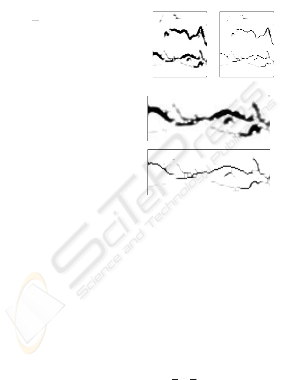
Spectrogram

Time

Frequency

0 0.5 1

300

750

1200

Image transformation

Time

Frequency

0 0.5 1

300

750

1200

Spectrogram

Image transformation

Figure 1: First row: Spectrogram and its transformation

with the PDE model. Subsequent plots: detail of the howl

contained within the range 300−750 Hz. We observe the IF

concentration and smoothing effect of the PDE algorithm.

PDE based algorithm than if we simply threshold the

image spectrogram. This is due to the local applica-

tion of gaussian ﬁlters in regions of small gradients

(noise, among them) while anisotropic diffusion (in

the orthogonal direction to the gradient) is applied in

regions of large gradients (edges-IF lines). Therefore,

a possible way to improve the image obtained by the

differential reassigned spectrogram is modifying (6)

by adding a diffusive term with the mentioned prop-

erties.

Let us make a ﬁnal observation before writing the

model we work with. In the derivation of both the re-

assigned and the differential reassigned spectrogram

the property of energy conservation is imposed, im-

plying that energy values on ridges increase. Indeed,

let B be a neighborhood of a point of maximum for

, in which divr = ∆logu

< 0, and let (t

,ω

) ∈ B.

Let χ

(t,ω,τ) denote the characteristic deﬁned by (5)

starting at (t

,ω

). Evaluating Eq. (6) along χ

obtain

dτ

u =

∂u

∂τ

+ r· ∇u = −udivr, (9)

implying that u experiments exponential increase in

NOISE REDUCTION AND VOICE SEPARATION ALGORITHMS APPLIED TO WOLF POPULATION COUNTING

B. For image processing, it is desirable the maximum

principle to hold, i.e., that the bounds minu

≤ u ≤

maxu

hold for any (t,ω,τ) ∈ Ω× R

, ensuring that

the processed image lies within the range of image

deﬁnition ([0,255], usually). A simple way, which we

shall address, to ensure this property is by dropping

the right hand side term of Eq. (9), i.e., replacing Eq.

(6) by the transport equation

∂u

∂τ

+ r· ∇u = 0. (10)

However, no energy conservation law will apply any-

more (note that u is constant along the character-

istics). The combination of the differential reas-

signment problem with the edge-detection image-

smoothing algorithm (L.

Alvarez, 1992) is written as

∂u

∂τ

∇log(u

) · ∇u− g(|G

∗ ∇u|)A(u) = 0, (11)

in Ω × R

, together with the boundary data (8) and

the initial condition (7). Parameter ε ≥ 0 allows us

to play with different balances between transport and

diffusion effects. The diffusion operator is given by

A(u) = (1−h(|∇u|))∆u+h(|∇u|)

∑

j=1,...,n

(

∇u

|∇u|

)

∂

∂x

Let us brieﬂy remind the properties and meaning of

the diffusive term components in equation (11):

• Function G

is a Gaussian of variance s. The vari-

ance is a scale parameter which ﬁxes the minimal

size of the details to be kept in the processed im-

age.

• Function g is non-increasing with g(0) = 1 and

g(∞) = 0. It is a contrast function, which allows

to decide whether a detail is sharp enough to be

kept.

• The composition of G

and g on ∇u rules the

speed of diffusion in the evolution of the image,

controlling the enhancement of the edges and the

noise smoothing.

• The diffusion operator A combines isotropic and

anisotropic diffusion. The ﬁrst smoothes the

image by local averaging while the second en-

forces the diffusion only on the orthogonal di-

rection to ∇u (along the edges). More precisely,

for θ

= ( j − 1) ∗ π/n, j = 1,... , n we deﬁne x

as the orthogonal to the direction θ

, i.e., x

−tsinθ

+ ωcosθ

. Then, smooth non-negative

functions f

(cosθ,sinθ) are designed to be ac-

tive only when θ is close to θ

. Therefore, the

anisotropic diffusion is taken in an approximated

direction to the orthogonal of ∇u. The combina-

tion of isotropic and anisotropic diffusions is con-

trolled by function h(s), which is nondecreasing

with

h(s) =



0 for s ≤ h

1 for s ≥ 2h

(12)

being h

the enhancement parameter.

In Fig. 1 we show an example of the outcome of our

algorithm for a signal composed by two howls. See

(B. Dugnol, 2007d; B. Dugnol, 2007c) for more de-

tails and other numerical experiments.

3 HOWL TRACKING AND

SEPARATION

A wolves chorus is composed, mainly, by howls and

barks which, from the analytical point of view, may

be regarded as chirp functions. The former has a long

time support and a small frequency range variation,

while the latter is almost punctually localized in time

but posses a large frequency spectrum. It is conve-

nient, therefore, adopting a parametric model to rep-

resent the wolveschorus as an addition of chirps given

by the function f : [0,T] → C,

f(t) =

∑

n=1

(t)exp[iφ

(t)], (13)

with T the length of the chorus emission, a

and φ

the chirps amplitude and phase, respectively, and with

N, the number of chirps contained in the chorus. We

notice that N is not necessarily the number of wolves

since, for instance, harmonics of a given fundamental

tone are counted separately.

To identify the unknowns N, a

and φ

we pro-

ceed in two steps. Firstly, for a time discretization of

the time interval [0,T], sayt

, for j = 0,..., J, we pro-

duce estimates of the amplitude a

) and the phase

) of the chirps contained at such discrete times.

Secondly, we establish criteria which allow us decid-

ing if the computed estimates at adjacent times do be-

long to the same global chirp or do not.

For the ﬁrst step we use the Chirplet transform de-

ﬁned by

Ψf (t

,ξ,µ;λ) =

∞

−∞

f (t)ψ

,ξ,µ,λ

(t)dt, (14)

with the complex window ψ

,ξ,µ,λ

given by

,ξ,µ,λ

(t) = v

(t − t

)exp

i(ξt +

(t − t

)

(15)

Here, v ∈ L

(R) denotes a real window, v

(·) =

v(·/λ), with λ > 0, and the parameters t

,ξ,µ ∈ R,

stand for time, instantaneous frequencyand chirp rate,

respectively. The quadratic energy distribution corre-

sponding to the chirplet transform (14) is given by

f(t

,ξ,µ;λ) = |Ψf (t

,ξ,µ;λ)|

. (16)

BIOSIGNALS 2008 - International Conference on Bio-inspired Systems and Signal Processing

For a linear chirp of the form

f(t) = a(t) exp[i(

(t −t

)

+ β(t −t

) + γ)],

it is straightforward to prove that the energy dis-

tribution (16) has a global maximum at (α,β), al-

lowing us to determine the IF and chirp rate of a

given linear chirp by localizing the maxima of the en-

ergy distribution. For more general forms of mono-

component chirps we have the following localization

result (B. Dugnol, 2007b)

Theorem 1 Let f (t) = a(t)exp[iφ(t)], with a ∈

(R) non-negative and φ ∈ C

(R). For all ε > 0

and ξ,µ ∈ R there exists L > 0 such that if λ < L then

f (t

,ξ,µ;λ) 6 ε+ P



,φ

′

),φ

′′

);λ



(17)

In addition,

lim

λ→0



,φ

′

),φ

′′

);λ



= a(t

)

. (18)

In other words, for a general mono-component chirp

the energy distribution maximum provides an arbi-

trarily close approximation to the IF and chirp rate

of the signal. Moreover, its amplitude may also be es-

timated by shrinking the window time support at the

maximum point.

Finally, for a multi-component chirp f (t) =

∑

n=1

(t)exp[iφ

(t)] the situation is somehow more

involved since although the energy distribution still

has maxima at (φ

′

),φ

′′

)) for all n such that

) 6= 0, these are now of local nature, and in fact,

spurious local maxima not corresponding to any chirp

may appear due to the energy interaction among the

actual chirps.

4 NUMERICAL EXPERIMENTS

According to the recording quality, we start our algo-

rithm enhancing the signal with the PDE algorithm

explained in Section 2 or directly with the separa-

tion algorithm introduced in Section 3. For details

about the implementation of the former, we refer the

reader to (B. Dugnol, 2007c). Following, we brieﬂy

comment about the separation algorithm implementa-

tion. We start by computing the energy distribution,

f (τ

,ξ,µ;λ) at a set of discrete times τ

= m∗ τ

of constant time step, τ, and for a ﬁxed window width

λ. Next we compute the maxima of the energy at each

of these times. When the signal is mono-component

or the various components of the signal are far from

each other relative to the window width, the maxima

of P

correspond to some (φ

′

(τ

),φ

′′

(τ

)) which are

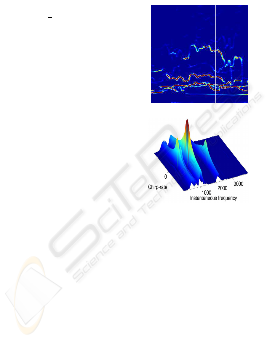
0.5 1 1.5 2 2.5

1000

2000

3000

4000

Time

Frequency

Figure 2: Above: STFT of a ﬁeld recorded signal. Be-

low: quadratic energy distribution of the chirplet transform

at t

= 2. Maxima correspond to IF and chirp rate chirps

locations. We observe the different behavior in the ξ and µ

directions at these maxima.

then identiﬁed as the IF and chirp-rate of a chirp can-

didate. However, when multi-component signals are

close to each other or are crossing, some spurious lo-

cal maxima are produced which do not correspond to

any actual chirp. Therefore, some criterium must be

used to select the correct local maxima at each τ

Although we lack of an analytical proof, there are ev-

idences suggesting that maxima produced by chirps,

i.e., at points of the type (φ

′

(τ

),φ

′′

(τ

)), decrease

much faster in the ξ direction than in the µ direction,

see Fig. 2, a phenomenon that does not occur at spuri-

ous maxima. We use this fact to choose the candidates

ﬁrst by selecting ξ

, for k = 1,. ..,K, which are max-

ima for

sup

f (τ

,ξ,µ;λ),

and, among them, selecting the maxima with re-

spect to µ of P

f (τ

,ξ

,µ;λ). We ﬁnally establish

a threshold parameter to ﬁlter out possible local max-

NOISE REDUCTION AND VOICE SEPARATION ALGORITHMS APPLIED TO WOLF POPULATION COUNTING

ima located at points that do not correspond to any

′

(τ

) but which are close to two of them. We set

this threshold such that the existence of two consecu-

tive maxima is avoided.

In this way we obtain, for each τ

, a set of points

(µ

,ξ

), for i

= 1,..., I

, which correspond to the

IF’s and chirp-rates of chirps with time support in-

cluding τ

The next step is the chirp separation. We note that

if the time step τ = τ

m+1

− τ

is small enough, then

m+1

− τ

m+1

≈ ξ

+ τ

Introducing a new parameter, ν, we test this property

by imposing the condition

2ξ

m+1

− τµ

m+1

2ξ

+ τµ

< ν, (19)

for two points to be in the same chirp. In the experi-

ments we take ν = 2

1/13

≈ 1.0548.

Finally, in the case in which test (19) is satisﬁed

by more than one point, i.e., when there exist points



m+1

,µ

m+1



and



m+1

,µ

m+1



such that (19) holds

for the same (ξ

,µ

), we impose a regularity cri-

terium and choose the point with a closer chirp-rate

to that of (ξ

,µ

). This is a situation typically aris-

ing at chirps crossings points.

Summarizing, the chirp separation algorithm is

implemented as follows:

• Each point (ξ

,µ

), for i

= 1,. ..,I

, is assumed

to belong to a distinct chirp.

• For k = 2,3,..., we use the described criteria to

decide if



,µ



, for : i

= 1, ...,I

, belongs to

an already detected chirp. On the contrary, it is

established as the starting point of a new chirp.

• When the above iteration is ﬁnished and to avoid

artifacts due to numerical errors, we disregard

chirps composed by a unique point.

Finally, once the chirps are separated, we use the fol-

lowing approximation, motivated by Theorem 1, to

estimate the amplitude

a(τ

)

≈

λ[bv(0)]



,φ

′

(τ

),φ

′′

(τ

);λ



Again, to avoid artifacts due to numerical discretiza-

tion, we neglect portions of signals with an amplitude

lower than certain relative threshold , ε ∈ (0,1), of the

maximum amplitude of the whole signal, considering

that in this case no chirp is present.

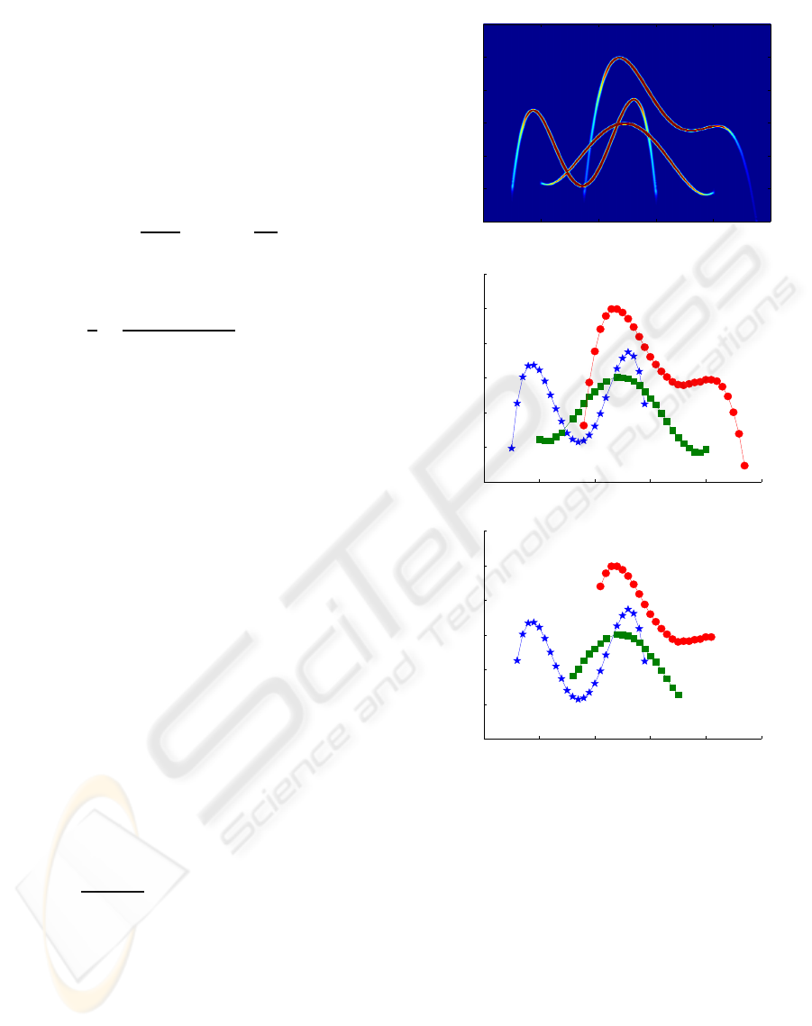
4.1 Experiment 1. A Synthetic Signal

In this ﬁrst experiment we test our algorithm with a

synthetic signal, f, composed by the addition of three

Time

Frequency

Spectrogram

0 2 4 6 8 10

250

500

750

1000

1250

1500

0 2 4 6 8 10

250

500

750

1000

1250

1500

Time

Frequency

0 2 4 6 8 10

250

500

750

1000

1250

1500

Time

Frequency

Figure 3: Spectrogram of the clean signal and results of

the chirp localization and separation algorithm for clean and

noisy signals, respectively.

nonlinear chirps (spectrogram shown in Fig. 3) and

with the same signal corrupted with an additive noise

of similar amplitude than that of f , i.e., with SNR= 0.

We used the same time step, τ = 0.2 sec, and

window width, λ = 0.1 sec, to process both signals,

while we set the relative threshold amplitude level to

ε = 0.01 for the clean signal and to ε = 0.1 for the

noisy signal. The results of our algorithm of denois-

ing, detection and separation is shown in Fig. 3. We

observe that for the clean signal all chirps are cap-

tured with a high degree of accuracy even at cross-

ing points. We also observe that the main effect of

noise corruption is the lose of information at chirps

BIOSIGNALS 2008 - International Conference on Bio-inspired Systems and Signal Processing

low amplitude range. However, the number of them

is correctly computed.

In Fig. 4 we show the amplitude, IF and chirp-

rate estimations of the chirp which is more affected by

the noise corruption, for both clean and noisy signals.

The main effect of noise corruption is observed in the

amplitude computation and in the lose of information

in the tails of the three quantities.

0 2 4 6 8 10

0.1

0.2

0.3

0.4

0.5

Chirp 3

Time

Analytic amplitude

0 2 4 6 8 10

0.1

0.2

0.3

0.4

0.5

Chirp 3

Time

Analytic amplitude

0 2 4 6 8 10

250

500

750

1000

1250

1500

Chirp 3

Time

Instantaneous frequency

0 2 4 6 8 10

250

500

750

1000

1250

1500

Chirp 3

Time

Instantaneous frequency

0 2 4 6 8 10

−2000

−1000

1000

2000

Chirp 3

Time

Chirp−rate

0 2 4 6 8 10

−2000

−1000

1000

2000

Chirp 3

Time

Chirp−rate

Figure 4: Amplitude, IF and chirp rate for the clean signal

(left column) and noisy signal (right column). Solid lines

correspond to exact values and crosses to computed values.

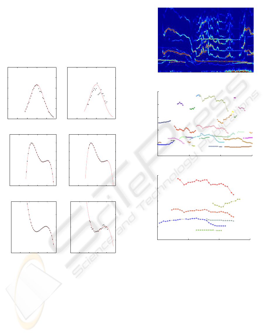
1 2 3 4

500

1000

1500

2000

2500

Time

Frequency

Spectrogram

0 1 2 3

500

1000

1500

2000

2500

Time

Frequency

Howl−tracking result

1 1.5 2 2.5

500

1000

1500

2000

2500

Time

Frequency

Howl−tracking result

Figure 5: First row: spectrogram of the ﬁeld recorded signal

utilized in Experiment 2. Second row: result of the chirp lo-

calization and separation algorithm. Third row: a zoom of

the previous plot showing six separated chirps correspond-

ing to ﬁve wolves howls.

4.2 Experiment 2. A Field Recorded

Wolves Chorus

In this experiment we analyze a rather complex signal

obtained from ﬁeld recordings of wolves choruses in

wilderness, (L. Llaneza, ). Due to the noise present

in the recording, we ﬁrst use the PDE algorithm to

enhance the signal and reduce the noise, see (B. Dug-

nol, 2007c) for details. For the separation algorithm,

we ﬁxed the time step as τ = 0.03 sec, the relative am-

NOISE REDUCTION AND VOICE SEPARATION ALGORITHMS APPLIED TO WOLF POPULATION COUNTING

plitude threshold as ε = 0.01 and the window width as

λ = 0.0625 sec.

The algorithm output is composed by 32 chirps

which should correspond to the howls and barks (with

all their harmonics) emitted by the wolves along the

duration of the recording (about ﬁve sec). The result

is shown in Fig. 5. Since our aim is giving an estimate

of how many individuals are emitting in a recording,

we plot a zoom of the separating algorithm result for

the time interval (1, 2.5). Here, the number of chirps

reduces to six. However, it seems that one couple of

them are harmonics, the couples formed by the chirp

around 1000 Hz and the highest IF chirp. Therefore,

we may conclude that at least ﬁve wolves are emitting

in this interval of time. A similar analysis is carried

out with other time subintervals until all the recorded

signal is analyzed.

5 CONCLUSIONS

A combined algorithm for signal enhancement and

voice separation is utilized for wolf population count-

ing. Although ﬁeld recorded wolf chorus signals

posses a complex structure due to noise corruption

and nonlinear multi-component character, the out-

come of our algorithm provides us with accurate es-

timates of the number of individuals emitting in a

given recording. Thus, the algorithm seems to be a

good complement or, even, an alternative to existent

methodologies, mainly based in wolf traces collection

or in the intrusive attaching of electronic devices to

the animals. Clearly, our algorithm is not limited to

wolves emissions but to any signal which may reason-

ably be modelled as an addition of chirps, opening its

utilization to other applications. Drawbacks of the al-

gorithm are related to the expert dependent election of

some parameters, such as the amplitude threshold, or

to the execution time when denoising and separation

of long duration signals must be accomplished. We

are currently working in the improvement of these as-

pects as well as in the recognition of components cor-

responding to the same emissor, such as harmonics of

a fundamental chirp, pursuing the full automatization

of the counting algorithm.

ACKNOWLEDGEMENTS

The ﬁrst three authors are supported by Project

PC0448, Gobierno del Principado de Asturias, Spain.

Third and fourth authors are supported by the Spanish

DGI Project MTM2004-05417.

REFERENCES

Auger, F. (1991). Repr´esentation temps-fr´equence des sig-

naux non-stationnaires: Synthe`ese et contributions.

th`ese de doctorat, Ecole Centrale de Nantes.

B. Dugnol, C. Fern´andez, G. G. (2007a). Wolves counting

by spectrogram image processing. Appl. Math. Com-

put., 186:820–830.

B. Dugnol, C. Fern´andez, G. G. J. V. (2007b). Implementa-

tion of a chirplet transform method for separating and

counting wolf howls. Preprint 1, Dpt. Mathematics,

Univ. of Oviedo, Spain.

B. Dugnol, C. Fern´andez, G. G. J. V. (2007c). Implemen-

tation of a diffusive differential reassignment method

for signal enhancement. an application to wolf pop-

ulation counting. Appl. Math. Comput. To appear.

E-version: doi:10.1016/j.amc.2007.03.086.

B. Dugnol, C. Fern´andez, G. G. J. V. (2007d). On pde-

based spectrogram image restoration. application to

wolf chorus noise reduction and comparison with

other algorithms. In E. Damiani, A. Dipanda, K.

Y. L. L. P. S., editor, Signal processing for image

enhancement and multimedia processing, volume 34

of Multimedia systems and applications. Springer

Verlag. To appear. (e-version in http://www.u-

bourgogne.fr/SITIS/06/Proceedings/index.htm).

E. Chassandre-Mottin, I. Daubechies, F. A. P. F. (1997).

Differential reassignment. IEEE Signal Processing

Letters, 4(10):293–294.

F. Auger, P. F. (1995). Improving the readability of

time-frequency and time-scale representations by the

method of reassignment. IEEE Trans. Signal Process-

ing, 43(5):1068–1089.

H. M. Ozaktas, Z. Zalevsky, M. A. K. (2001). The Frac-

tional Fourier Transform with Applications in Optics

and Signal Processing. Wiley, Chichester.

K. Kodera, R. Gendrin, C. d. V. (1978). Analysis of time-

varying signals with small bt values. IEEE Trans-

actions on Acoustics, Speech and Signal Processing,

26(1):64–76.

Alvarez, P. L. Lions, J. M. M. (1992). Image selective

smoothing and edge detection by nonlinear diffusion.

ii. SIAM J. Numer. Anal., 29(3):845–866.

L. Angrisani, M. D. (2002). A measurement method based

on a modiﬁed version of the chirplet transform for

instantaneous frequency estimation. IEEE Trans. In-

strum. Meas., 51:704–711.

L. Llaneza, V. P. Field recordings obtained in wilderness

in asturias (spain) in the 2003 campaign. Asesores en

Recursos Naturales, S.L.

Mallat, S. (1998). A wavelet tour of signal processing. Aca-

demic Press, London.

S. Mann, S. H. (1995). The chirplet transform: Physi-

cal considerations. IEEE Trans. Signal Processing,

43(11):2745–2761.

Skonhoft, A. (2006). The costs and beneﬁts of ani-

mal predation: An analysis of scandinavian wolf re-

colonization. Ecological Economics, 58(4):830–841.

BIOSIGNALS 2008 - International Conference on Bio-inspired Systems and Signal Processing