AN INSERTION STRATEGY FOR A TWO-DIMENSIONAL

SPATIAL ACCESS METHOD

Wendy Osborn

Department of Mathematics and Computer Science, University of Lethbridge, Lethbridge, Alberta, Canada, T1K 3M4

Ken Barker

Department of Computer Science, University of Calgary, Calgary, Alberta, Canada, T2N 1N4

Keywords:

Spatial access methods, multidimensional, hierarchical, data structures, performance.

Abstract:

This paper presents the 2DR-tree, a novel approach for accessing spatial data. The 2DR-tree uses nodes

that are the same dimensionality as the data space. All spatial relationships between objects are preserved.

A validity rule ensures that every node preserves the spatial relationships among its objects. The proposed

insertion strategy adds a new object by recursively partitioning the space occupied by a set of objects. A

performance evaluation shows the advantages of the 2DR-tree and identiﬁes issues for future consideration.

1 INTRODUCTION

A spatial database contains a large collection of ob-

jects that are located in multidimensional space. An

important research issue in spatial databases is the ef-

ﬁcient retrieval of objects based on location, using

spatial access methods (SAMs).

No n-dimensional to one-dimensional mapping of

spatial data exists that preserves all spatial relation-

ships between objects (Gaede and G

unther, 1998).

However, SAMs use approaches that are intended for

alphanumeric data. This leads to a one-dimensional

spatial organization of objects. This also leads to un-

necessary searching within a node and the data struc-

ture as a whole, because the only option is a linear

search of a node in its entirety. It is not possible to

search only part of a node.

This paper describes a portion of our work on

a new hierarchical SAM to alleviate this limitation.

The 2DR-tree ﬁts the existing object space by using

nodes of the same dimensionality. Therefore, two-

dimensional nodes are used to index objects in two-

dimensional space. Objects in each node are orga-

nized using a validity rule that preserves all spatial re-

lationships. This strategy allows the 2DR-tree to sup-

port non-linear searching strategies. We expect that

this strategy will reduce the amount of searching that

is performed in a node. In addition, overcoverage and

overlap will also be reduced.

2 RELATED WORK

Many approaches for indexing objects based on lo-

cation are proposed in the literature (see (Gaede and

unther, 1998; Samet, 1990; Shekhar and Chawla,

2003) for surveys). These approaches are classi-

ﬁed into three categories (Gaede and G

unther, 1998):

main memory methods, point access methods and

spatial access methods (SAMs). Many important

strategies are proposed in all categories. We focus on

SAMs, since our work is in this category.

SAMs provide uniform access to both point and

object data. Also, they remain height-balanced in the

presence of a dynamic object set. Many SAMs are

proposed in the literature (Guttman, 1984; Beckmann

et al., 1990; Berchtold et al., 1996; Kamel and Falout-

sos, 1994; Sellis et al., 1987; Orenstein and Merrett,

1984; Koudas, 2000). They can be classiﬁed (Gaede

and G

unther, 1998) into approximation, clipping, and

mapping methods.

Approximation methods store a hierarchy of ap-

proximations of both objects and the space occu-

pied by subsets of objects. Since the space is not

partitioned, approximations can overlap. Many ap-

proximation methods are proposed, including the R-

tree (Guttman, 1984), the R

∗

-tree (Beckmann et al.,

1990) and the X-tree (Berchtold et al., 1996). Clip-

ping methods, such as the R

-tree (Sellis et al.,

1987), partition an object into parts so that over-

295

Osborn W. and Barker K. (2007).

AN INSERTION STRATEGY FOR A TWO-DIMENSIONAL SPATIAL ACCESS METHOD.

In Proceedings of the Ninth International Conference on Enterprise Information Systems - DISI, pages 295-300

DOI: 10.5220/0002408002950300

 SciTePress

lap is avoided. Mapping methods map objects in n-

dimensional space into a one-dimensional order. The

objects are then stored and retrieved using an access

method such as a B

-tree (Comer, 1979). Approaches

that use mapping include Z-ordering (Orenstein and

Merrett, 1984), the Hilbert R-tree (Kamel and Falout-

sos, 1994), and the Filter tree (Koudas, 2000).

No n-dimensional to one-dimensional mapping

of spatial data exists that preserves all spatial re-

lationships between objects (Gaede and G

unther,

1998). A limitation to hierarchical SAMs is their

one-dimensional structure. This forces objects in n-

dimensional space into a one-dimensional ordering,

which results in the loss of spatial relationships. This

leads to inefﬁcient searching, both within a node and

the structure as a whole, because the only option is a

linear search of a node in its entirety. Mapping meth-

ods do provide a one-dimensional ordering of objects,

but they cannot maintain all spatial relationships.

3 THE 2DR-TREE

The 2DR-tree is an approximation SAM that uses

nodes that are two-dimensional in structure to orga-

nize approximations for objects and the space oc-

cupied by objects. In every node, an approxima-

tion is stored in an appropriate location with re-

spect to all other approximations in the node. Using

two-dimensional nodes allows approximations to be

placed so that spatial relationships are preserved. We

present the 2DR-tree and deﬁne key concepts below.

3.1 Preliminaries

The 2DR-tree uses a minimum bounding rectangle

(MBR) for approximating an object and the space oc-

cupied by a subset of objects. An MBR is the mini-

mum extent along both the x-axis and the y-axis that

encompasses an object in a leaf node, and a subset of

MBRs in a non-leaf node. The centroid of an MBR

are the co-ordinates (i, j) of its centre.

The supported spatial relationships are north, east,

south, west, northeast, northwest, southeast, and

southwest. A spatial relationship is determined by

comparing the centroids between two MBRs. This

leads to a smaller set than that in (Papadias et al.,

1996), but we feel this simpler technique covers all

required cases.

The coverage of an MBR is the total area covered

by the rectangle. The coverage of a tree is the total

coverage of all MBRs in the tree. The overcoverage

of an MBR is the area of the whitespace within a rect-

angle. The overcoverage of a tree is the total overcov-

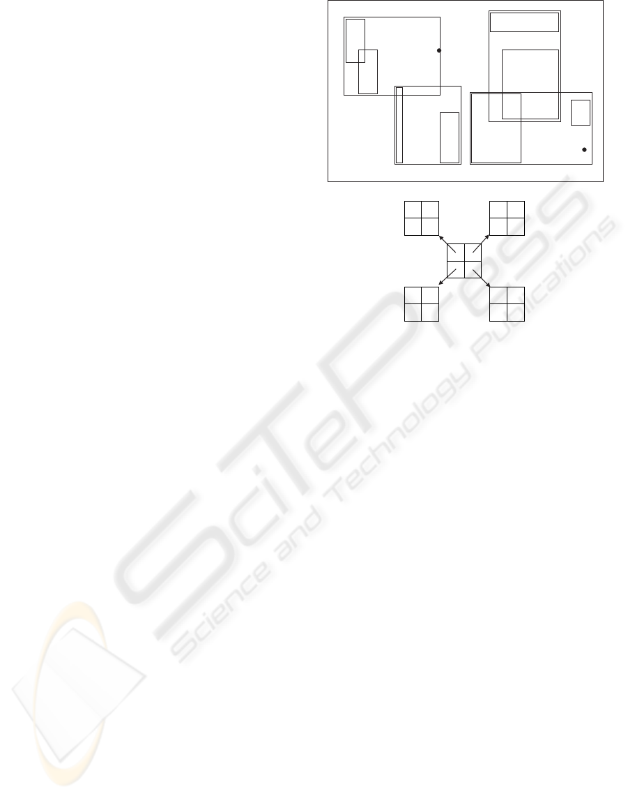
Figure 1: Order 4*4 2DR-tree.

erage of all MBRs in the tree. The overlap of a tree is

the total overlap between all pairs of MBRs.

For each node N, X is the number of indexed lo-

cations along the x-axis, and Y is the number of in-

dexed locations along the y-axis. The order of N is

O = X ∗ Y. All nodes in a 2DR-tree have the same

order. Therefore, the order of a 2DR-tree is the order

of its nodes. Each location (i, j) in node N stores:

(MBR

(i, j)

, ptr

(i, j)

)

where MBR

(i, j)

is an MBR and ptr

(i, j)

is a pointer. In

a leaf node, MBR

(i, j)

encloses an object and ptr

(i, j)

references the object on secondary storage. In a non-

leaf node, MBR

(i, j)

encloses all MBRs in the subtree

referenced by ptr

(i, j)

A node space is the area of space occupied by a

set of objects. This is equal to the MBR that encloses

the objects. A node region (lx, hx, ly, hy) is a two-

dimensional subset of (x, y) index locations in a node.

The index values lx and hx are the lower and upper

bounds of the node region along the x-axis. The in-

dex values ly and hy are the lower and upper bounds

of the node region along the y-axis.

3.2 Node Validity

To employ different searching strategies, the spa-

tial relationships between MBRs in each node must

be preserved. For each location N

(i, j)

, i = 0. . . (X −

ICEIS 2007 - International Conference on Enterprise Information Systems

296

1), j = 0. . . (Y − 1) in node N, if N

(i, j)

contains

MBR

(i, j)

• Location N

(k,l)

, k = (i + 1). . . (X − 1), l = 0. . . j

contains MBR

(k,l)

whose centroid is southeast of

the centroid for MBR

(i, j)

• Location N

(k,l)

, k = (i + 1) . . . (X − 1), l = ( j +

1). . . (Y − 1) contains MBR

(k,l)

whose centroid is

northeast of the centroid for MBR

(i, j)

, and

• Location N

(k,l)

, k = 0. . . i, l = ( j + 1) . . . (Y − 1)

contains MBR

(k,l)

whose centroid is northwest of

the centroid for MBR

(i, j)

Figure 1 shows an order 2*2 2DR-tree that pre-

serves all spatial relationships for the given data set

(from (Gaede and G

unther, 1998)). Beginning with

the leaf node descending from root location (0, 0), the

centroid for m3 is located southeast of the centroid so

m3 is located east of m4 in the node (m4,m3). In node

(m5,p5,m8), p5 is located southeast of the centroid for

m5, and the centroid for m8 is located northeast of the

centroid for m5 and northwest of p5. Therefore, p5 is

stored east of m5 while m8 is stored northeast of m5

and north of p5. Spatial relationships are also main-

tained in nodes (m7,m9), (m2,m1,p9), and the root

node.

4 2DR-TREE INSERTION

The 2DR-tree insertion strategy has ﬁve stages: 1)

search for an appropriate leaf node, 2) search for the

appropriate location within the leaf node, 3) place the

new object with respect to any objects remaining in

the node so that spatial relationships are maintained,

4) attempt to put back the objects that were removed

so that spatial relationships are maintained – if not

possible, then a split is performed, and 5) perform an

update of the insertion path. The ﬁrst four stages are

detailed here.

4.1 Leaf Node Search

An appropriate leaf node is found for new object

MBR

by applying a greedy search to each node on

the insertion path. Each chosen node contains an

MBR that requires either a minimal or the least area

increase necessary to include the new object. The

greedy search ﬁnds this MBR along a path of decreas-

ing area increases. The most optimal MBR may not

be found, but the number involved in the search is

reduced. This is because the approximations in the

node are now organized, and other search strategies

can now be applied.

Beginning at location (0, 0), each approximation

in location (i, j) on the search path is compared with

(i, j + 1),(i + 1, j + 1) and (i + 1, j). If the MBR at

(i, j) has the smallest area increase, the search termi-

nates in the node and continues in the corresponding

subtree. Otherwise, the search continues in the direc-

tion that contains an MBR with the smallest area in-

crease. This is repeated at each level of the tree, until

a leaf node is reached.

4.2 Object Location Search

After a leaf node is found, a location for MBR

found within the node by performing a recursive par-

tition of the node space NS that corresponds to the leaf

node. For each recursive stage, two steps take place.

First, the node space is partitioned into two equal sub-

spaces through the dimension with the longest extent.

Second, a node region that corresponds to each sub-

space is identiﬁed. The subspace (and corresponding

node region) that contains MBR

is selected for fur-

ther partitioning, while the node region correspond-

ing to the other subspace is removed from the node

and will be put back after MBR

is inserted.

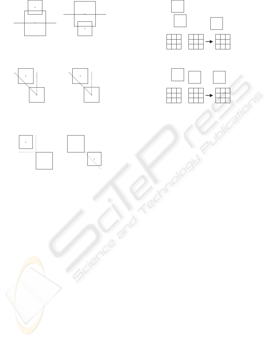
Figure 2 shows partitioning for the north and south

cases, and how the new object relates to the partition.

In Figure 2a, the new object N is located north of the

partition. In Figure 2b, N is located south of the par-

tition. In these cases, the north or south subspace re-

spectively is chosen for further partitioning.

Recursive partitioning continues until either one

MBR remains in the node (MBR

), or multiple objects

exist and MBR

has some speciﬁc spatial relationship

with those objects.

4.3 New Object Placement

After removing subsets of objects, MBR

is inserted

with respect to the remaining object(s) to ensure that

all spatial relationships are maintained. We present

the cases for insertion relative to one MBR, followed

by insertion relative to multiple MBRs.

The cases for insertion MBR

relative to one

remaining approximation, MBR

are listed below.

MBR

is located at (i, j).

North Insert. MBR

is located northwest of MBR

and the slope of a line between their centroids is less

than −1. MBR

is inserted in location (i, j+ 1). This

is depicted in Figure 3a.

North Swap Insert. MBR

is located southeast of

MBR

and the slope of a line between their centroids

is less than −1. MBR

is swapped with MBR

and

MBR

is inserted in location (i, j + 1). This is de-

picted in Figure 3b.

AN INSERTION STRATEGY FOR A TWO-DIMENSIONAL SPATIAL ACCESS METHOD

297

MBR

a. North b. South

Figure 2: Partitioning Cases for North and South.

MBR

a. North Insert b. North Swap Insert

Figure 3: Single Object Cases for North Inserts.

MBR

a. North Insert b. East Insert

Figure 4: Multiple Object Cases for North and East.

East Insert. MBR

is located southeast of MBR

and

the slope of a line between their centroids is greater

than −1. MBR

is inserted in (i+ 1, j).

East Swap Insert. MBR

is located northwest of

MBR

and the slope of a line between their centroids

is greater than −1. MBR

is swapped with MBR

and

MBR

is inserted in (i+ 1, j).

Northeast Insert. MBR

is located northeast of

MBR

. MBR

is inserted in (i+ 1, j + 1).

Northeast Swap Insert. MBR

is located northeast of

MBR

. MBR

is swapped with MBR

and MBR

inserted in (i+ 1, j + 1).

The multiple object cases identify situations

where MBR

has certain spatial relationships rela-

tive to all remaining approximations in the node.

For all cases, the remaining approximations occupy

node space NS, which corresponds to node region

(lx

rns

, hx

rns

, ly

rns

, hy

rns

North Insert. MBR

is located northwest of NS, and

the slope of a line between their centroids is less than

−1. MBR

is inserted in location (lx

rns

, hy

rns

+ 1).

This is depicted in Figure 4a.

East Insert. MBR

is located southeast of NS, and the

slope of a line between their centroids is greater than

2 2

a. East, No Overlap

2 2

b. East, Overlap

Figure 5: Node Restore for East Cases.

−1. MBR

is inserted in location (hx

rns

+ 1, ly

rns

This is depicted in Figure 4b.

Northeast Insert. MBR

is located northeast of NS.

MBR

is inserted in location (hx

rns

+ 1, hy

rns

+ 1).

Northeast Swap Insert. MBR

is located southwest

of NS. The node region is shifted to the northeast

(i.e. over one column and up one row), and MBR

inserted into the original (lx

rns

, ly

rns

) location.

4.4 Restoring the Leaf Node

After MBR

is inserted, any removed node regions

are restored in the reverse order of their removal. Af-

ter replacing each node region, a validity test is per-

formed. The ﬁnal result is either a completely re-

stored node, or a set of nodes if a split is required.

Each removed node region has a direction of

north, south, east, or west, depending on which side

of the partition its corresponding node space was on.

This direction is used to restore the node region rel-

ative to (lx

rns

, hx

rns

, ly

rns

, hy

rns

). When MBR

is in-

serted, one or both of the upper node region bound-

aries hx

rns

and hy

rns

are increased. When this in-

crease occurs, potential overlap problems arise be-

tween the node region (lx

rns

, hx

rns

, ly

rns

, hy

rns

) and

some removed node regions, namely the east and

north node regions. Therefore, the resulting cases

are north, north with overlap, east, east with overlap,

south and west.

The east and east with overlap cases are depicted

in Figure 5. When east node region (lx

, hx

, ly

, hy

)

does not overlap with (lx

rns

, hx

rns

, ly

rns

, hy

rns

), it is

put back into its original location. However, when the

east node region (lx

, hx

, ly

, hy

) does overlaps with

ICEIS 2007 - International Conference on Enterprise Information Systems

298

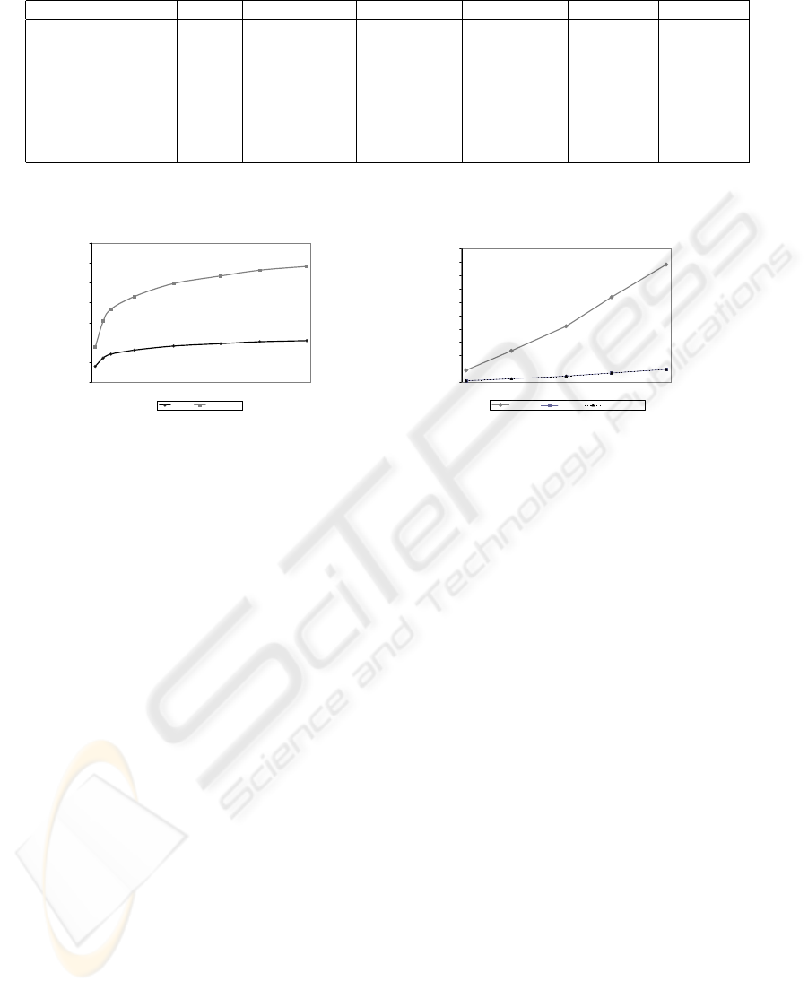
Table 1: Averages for Varying Object Set Size.

#Obj #Nodes Height Coverage Overcov Overlap #Seeks/Ins #Splits/Ins

100 127.97 8.10 128,906.74 15,801.81 13,070.12 17.82 1.04

500 654.06 12.31 1,233,595.22 138,768.90 129,630.80 30.74 1.12

1,000 1,312.53 14.19 3,232,169.34 355,257.04 340,590.69 36.74 1.13

2,000 2,619,52 16.23 8,784,155.25 959,547.75 935,355.26 43.11 1.13

4,000 5,244.69 18.26 23,448,427.79 2,535,300.42 2,494,116.09 49.59 1.13

6,000 7,867.63 19.47 41,887,513.70 4,525,004.07 4,465,319.16 53.43 1.13

8,000 10,470.28 20.44 63,752,968.22 6,862,775.80 6,792,707.51 56.28 1.13

10,000 13.077.67 21.00 88,158,132.24 9,517,985.63 9,432,726.01 58.20 1.13

#Object vs. Height and #Seeks/Ins

1000

2000

4000

6000

8000

10000

500

100

2000

10000

8000

6000

4000

500

100

#Objects

Height #Seeks/Ins

#Objects vs. Coverage/Overcoverage/Overlap

10000

8000

6000

4000

2000

4000

6000

8000

10000

100

Millions

#Objects

Coverage Overlap Overcoverage

a. #Objects vs. Height and #Seeks/Insert b. #Objects vs. Coverage/Overlap/Overcoverage

Figure 6: Affect of Object Set Size on Various Parameters.

(lx

rns

, hx

rns

, ly

rns

, hy

rns

), it is shifted one column east

from its original position before it is put back. The

other cases are handled similarly.

To handle overﬂow and node invalidity, different

splitting strategies are used. One strategy is the reduc-

tion split, which takes advantage of the node regions

that are removed from the node. Each node region

that cannot be put back is assigned to its own node.

5 PERFORMANCE EVALUATION

The preliminary performance evaluation observes the

behaviour of the 2DR-tree for different object set

sizes and distributions. We created object sets that

contain between 100 and 10,000 equal-sized squares.

With between 51-53% overlap, each set covers 67-

75% of the space.

Each test run constructs 1000 trees using random

sorts of the object set. The tree height, number of

nodes, average space utilization, coverage, overcov-

erage, overlap, average number of disk accesses per

insertion, and the average number of splits per in-

sertion are recorded. Each disk access retrieves one

node. We assume that each page from secondary stor-

age stores the information for one node, independent

of node size. We also assume that with the exception

of the root node and new nodes produced from a split,

each node is retrieved every time it is read. In the lat-

ter case, the MBRs required for updating are gener-

ated immediately after creating the node so retrieving

new nodes resulting from a split is not required.

We evaluate the insertion algorithm using the fol-

lowing sets of test runs: 1) varying the number of ob-

jects between 100 and 10000, using a 5x5 node size

and uniform distribution, 2) varying the data distri-

bution between uniform and exponential, using 500

objects and a 5x5 node size.

5.1 Results and Discussion

Table 1 shows the averages for each run when vary-

ing the number of objects inserted into the 2DR-tree.

The average number of seeks per insert is less than

three times the average tree height in all cases. This

includes the number required to ﬁnd the appropriate

leaf node so updating takes the remaining seeks. The

average number of seeks for updating is more than

one times the average tree height due to the average of

approximately one split per insertion occurring. This

is signiﬁcant since splits can be triggered by many sit-

uations in the 2DR-tree. The results show that splits

are not a signiﬁcant factor for 2DR-tree insertion.

Figure 6a shows the effect of the number of ob-

AN INSERTION STRATEGY FOR A TWO-DIMENSIONAL SPATIAL ACCESS METHOD

299

Table 2: Averages for Varying Distribution.

Distribution #Nodes Height Coverage Overcov Overlap #Seeks/Ins #Splits/Ins

Uniform 654.06 12.31 1,233,595.22 138,768.90 129,630.80 30.74 1.12

Exponential 652.63 12.31 638,430.98 64,157.58 67,130.08 30.71 1.10

jects inserted on the tree height, and the average num-

ber of disk accesses required for inserting an object.

Initially, the tree grows in height quickly but growth

slows signiﬁcantly as more objects are inserted. The

same occurs for the number of disk accesses.

Figure 6b shows the effect of the number of ob-

jects inserted on the coverage, overlap and overcover-

age. Results show that the coverage increases linearly

as the number of objects increase. In addition, the

rate of increase in overlap and overcoverage is signif-

icantly lower as the number of objects increase. Cov-

erage includes the object coverage, while overlap and

overcoverage are only calculated for non-leaf nodes.

One reason for the lower growth in overlap and over-

coverage is the ability of the 2DR-tree to “cluster”

objects located close together as the number of ob-

jects increase, which reduce both the overlap and the

wasted space in non-leaf approximations.

Table 2 shows the averages for each run when

varying the distribution of the data set. The results

show a signiﬁcant difference in coverage, overcover-

age, and overlap. The surprising result is that when

indexing exponentially distributed data, the 2DR-

tree achieves signiﬁcantly, almost 50%, lower cover-

age and overlap, and 54% lower overcoverage. The

height, number of nodes, and space utilization are not

a factor in this because they are not signiﬁcantly dif-

ferent between the data distributions. After many in-

sertions, “chains” that consist of many non-leaf nodes

that lead to one node with few objects - possibly one -

start to appear. An advantage to chains is that outliers

are separated from a cluster of objects, which reduces

the coverage, overcoverage, and overlap of MBRs.

6 CONCLUSION

This paper presents work on the 2DR-tree, which pre-

serves spatial relationships between all objects by us-

ing nodes that are the same dimensionality as the ob-

ject set. This structure supports non-linear search

strategies. We present the insertion strategy and some

preliminary evaluation results. The results show that

the 2DR-tree is ideal for larger objects sets with re-

spect to tree height. The average number of disk ac-

cesses and split per insert are reasonable. In addi-

tion, it is ideal for a dynamic skewed data set, which

achieves lower coverage, overcoverage, and overlap

than a dynamic, uniformly distributed data set.

Some research directions include: 1) a perfor-

mance evaluation versus other proposed SAMs; 2)

improving the average space utilization, which is very

low; 3) developing an algorithm for bottom-up tree

construction applicable to static data sets; 4) extend-

ing the 2DR-tree for three dimensions.

REFERENCES

Beckmann, N., Kriegel, H.-P., Schneider, R., and Seeger,

B. (1990). The R

∗

-tree: an efﬁcient and robust access

method for points and rectangles. In Proceedings of

the ACM SIGMOD International Conference on Man-

agement of Data, pages 322–31.

Berchtold, S., Keim, D., and Kriegel, H.-P. (1996). The X-

tree: An index structure for high-dimensional data. In

Proceedings of the 22nd International Conference on

Very Large Data Bases, pages 28–39.

Comer, D. (1979). The ubiquitous B-tree. ACM Computing

Surveys, 11:121–37.

Gaede, V. and G

unther, O. (1998). Multidimensional access

methods. ACM Computing Surveys, 30:170–231.

Guttman, A. (1984). R-trees: a dynamic index structure

for spatial searching. In Proceedings of the ACM

SIGMOD International Conference on Management

of Data, pages 47–57.

Kamel, I. and Faloutsos, C. (1994). Hilbert R-tree: an im-

proved r-tree using fractals. In Proceedings of the 20th

International Conference on Very Large Data Bases,

pages 500–9.

Koudas, N. (2000). Indexing support for spatial joins. Data

and Knowledge Engineering, 34:99–124.

Orenstein, J. and Merrett, T. (1984). A class of data struc-

tures for associative searching. In Proceedings of the

Third ACM SIGACT-SIGMOD Symposium on Princi-

ples of Database Systems, pages 181–90.

Papadias, D., Egenhofer, M., and Sharma, J. (1996). Hier-

archical reasoning about direction relations. In Pro-

ceedings of the 4th ACM-GIS.

Samet, H. (1990). The design and analysis of spatial data

structures. Addison-Wesley.

Sellis, T., Roussopoulos, N., and Faloutsos, C. (1987). The

-tree: a dynamic index for multi-dimensional ob-

jects. In Proceedings of the 13th International Con-

ference on Very Large Data Bases.

Shekhar, S. and Chawla, S. (2003). Spatial databases: a

tour. Prentice Hall.

ICEIS 2007 - International Conference on Enterprise Information Systems

300