PIN: A PARTITIONING & INDEXING OPTIMIZATION

METHOD FOR OLAP

Ricardo Jorge Santos

(1)

and Jorge Bernardino

(1, 2)

(1)

CISUC – Centre of Informatics and Systems of the University of Coimbra - University of Coimbra

(2)

ISEC – Superior Engineering Institute of Coimbra – Polytechnic Institute of Coimbra

Keywords: Optimizing, partitioning, indexing, data warehouse.

Abstract: Optimizing the performance of OLAP queries in relational data warehouses (DW) has always been a major

research issue. There are various techniques that can be used to achieve its goals, such as data partitioning,

indexing, data aggregation, data sampling, redefinition of database (DB) schemas, among others. In this

paper we present a simple and easy to implement method which links partitioning and indexing based on

the features present in predefined major decision making queries to efficiently optimize a data warehouse’s

performance. The evaluation of this method is also presented using the TPC-H benchmark, comparing it

with standard partitioning and indexing techniques, demonstrating its efficiency with single and multiple

simultaneous user scenarios.

1 INTRODUCTION

Performance optimization in data warehousing

(DWH) is always an important research issue. There

are various techniques which can be used for OLAP

performance optimization of relational databases

such as, among others: 1) Partitioning (Bellatreche,

2000), which reduces the data to scan for each

OLAP query; 2) Materialized Views (Agrawal,

2000), (Baralis, 1997) (Gupta, 1999), which store

summarized data and pre-calculated attributes, also

aiming to reduce the data to be scanned and

reducing time consumption for calculating aggregate

functions; 3) Indexing (Chaudhuri, 1997) (Chee-

Yong, 1999) (Gupta, 1997), which speeds up

processes such as accessing and filtering data; 4)

Data Sampling (Furtado, 2002), giving approximate

answers to queries based on representative samples

of subsets of data instead of having to scan the entire

data; 5) Redefinition of DB schemas (Vassiliadis,

1999) (Bizarro, 2002), trying to improve data

distribution and/or access by seeking efficient table

balancing; 6) Hardware optimization, such as

memory and CPU upgrading, distributing data

through several physical drives, etc.

In our opinion, sampling should not be preferred, for

it has an implicit statistical error margin attached

and almost never supplies an accurate answer

according to whole original data. Using materialized

views is often considered as a good technique, but it

has a big disadvantage. Since they consist on

aggregating the data to a certain level, they have

limited generic usage and each materialized view is

usually built for speeding up one or two queries

instead of the whole set of usual decision or ad-hoc

queries. Furthermore, they may take up much

physical space and increase DB maintenance efforts.

Hardware improvements for optimization issues is

not part of the scope of this paper, neither is

changing the data structures in the DW’s schema(s).

Although much work has been done with these

techniques separately, few have focused on their

combination (Bellatreche, 2004) (Bellatreche, 2002).

The author in (Sanjay, 2004) states that decision

making OLAP queries which are executed

periodically at regular intervals is by far the most

used form of obtaining decision making information.

This implies that this type of information is based

almost always on the same regular SQL instructions.

In this work we present an efficient alternative

method for a partitioning and indexing schema

aiming to optimize the DW’s global performance.

This method is based on analyzing the existing

features within the SQL OLAP queries which are

assumed as the DW’s main decision making queries.

The rest of this paper is organized as follows. In

170

Jorge Santos R. and Bernardino J. (2007).

PIN: A PARTITIONING & INDEXING OPTIMIZATION METHOD FOR OLAP.

In Proceedings of the Ninth International Conference on Enterprise Information Systems - DISI, pages 170-177

DOI: 10.5220/0002398301700177

 SciTePress

section 2, we refer issues and existing solutions

related to relational DW performance optimization

using partitioning and/or indexing. In section 3 we

present our optimization method. In section 4 we

illustrate an experimental evaluation of our method

using the TPC-H benchmark, and the final section

contains concluding remarks and future work.

2 RELATED WORK

DWH technology uses the relational data schema for

modeling the data in a warehouse. The data can be

modeled either using the star schema or the

snowflake schema. In this context, OLAP queries

require extensive join operations between fact and

dimension tables (Bellatreche, 2004). Several

optimization techniques have been proposed to

improve query performance, such as materialized

views (Agrawal, 2000) (Baralis, 1997) (Bellatreche,

2000B) (Gupta, 1999), advanced indexing

techniques using bitmapped indexes, join and

projection indexes (Agrawal, 2000) (Chaudhuri,

1997) (Chee-Yong, 1999) (Gupta, 1997) (O’Neil,

1997), and data partitioning (Bellatreche, 2000)

(Bellatreche, 2002) (Kalnis, 2001) (Sanjay, 2004),

among others.

The authors in (Agrawal, 2000) automatically

choose an appropriate set of materialized views and

consequent indexes from the workload experienced

by the system. This solution is integrated within the

Microsoft SQL Server 2000 DBMS’s tuning wizard.

In (Gupta, 1999) a maintenance-cost based selection

is presented for selecting which materialized views

should be built. In (Chaudhuri, 1997) (Chee-Yong,

1999) (Gupta, 1997) authors illustrate features on

which types of indexing should be performed based

on system workload, attribute cardinality and other

data characteristics. The work in (Bellatreche, 2005)

presents a genetic algorithm for schema

fragmentation selection, focused on how to fragment

the fact table based on the dimension table’s

partitioning schemas. Fragmenting the DW as a way

of speeding up multi-way joins and reducing query

execution cost is another possible optimization

method, as shown in (Bellatreche, 2000). In (Sanjay,

2004) the authors propose novel techniques for

designing a scalable solution as how to adequately

incorporate partitioning with DB design. In

(Bellatreche, 2004) the authors obtain tuning

parameters for better use of data partitioning, join

indexes and materialized views to optimize the cost

in a systematic usage form.

As stated previously, we discard materialized

views because of their poor general application for a

considerably large set of major queries, hence the

number of necessary materialized views is

proportional to the number of different queries.

Furthermore, the significant amount of space they

might take up in the DB is also a negative aspect,

along with increase of maintenance costs. Therefore,

we focus our work on two major performance

techniques for an alternative optimization schema:

partitioning and indexing. Considering that the most

efficient techniques rely on those which minimize

the amount of data to be scanned for producing each

major query’s response, our method proposes how

to implement an efficient partitioning schema and

consequent best practice indexing based on the

features presented in that set of the DW’s major

queries. Our method also minimizes DB

maintenance effort by defining an efficient number

of partitions per table, for an excessive amount of

partitions may result in poor performance

(Bellatreche, 2005).

3 PIN OPTIMIZATION METHOD

In order to guarantee data validation and integrity,

we advise maintaining the DB schema’s primary

keys and referential integrity constraints. Our PIN

(Partitioning and INdexing) method aims for

determining the best fragmentation attribute for each

table and how many fragments should be defined,

according to an overall ratio that combines all the

major OLAP query restriction predicates and

execution time, as well as all attribute’s cardinality.

This will accelerate OLAP queries having restriction

predicates on that attribute.

3.1 Defining the Partitioning Attributes

The first type of performance measurement we need

for our method is to evaluate the percentage for the

total number of records in each table in relation to

the total number of records which exist in the DW,

which will be used as a ratio for our method.

Consider c

as the number of existing records

within table T

and Σc

as the total number of

existing records within the DW. The percentage of

records for T

in the DW (ratio RPI

) is given by:

Σc

Another type of performance measure to

consider for our method is the impact of each

RPI

PIN: A PARTITIONING & INDEXING OPTIMIZATION METHOD FOR OLAP

171

isolated query execution time in the total time

needed for executing a workload with all of the

major queries. Consider t

as the average execution

time for each main DW query Q

, and Σt

as the

average execution time of the workload with all the

selected major queries. To obtain the percentage of

time corresponding to the execution of query Q

compared with the time spent in the execution of all

queries, representing another ratio for our method,

we can calculate the total time percentage impact for

each query (ratio TIP

) by:

Σt

We also need to know the impact given by the

number of records to be scanned related to each

attribute filtered values defined in the WHERE

clause of each OLAP query instruction. For

example, suppose a common sales table with a

record data structure (Sale_ID, Sale_Customer_ID,

Sale_Date, Sale_Amount) and an OLAP query in

which we needed to filter the sales records only with

attribute Sale_Date between [1-1-2006; 31-1-2006]

in order to produce the query’s answer. If the sales

table has a total of 100.000 records and there are

1.000 records which comply with the filtered

Sale_Date desired values, then the percentage of

interesting records within the sales table would be

equal to 1.000 / 100.000 = 0,01 in this particular

OLAP query. Consider an attribute A

belonging to a

table T

existing in the WHERE clause of a query Q

defining an interval of absolute values [I

; I

] for

including records in that query’s processing.

Consider c

as the total number of records of T

and

as the number of records in T

where the

recorded values of A

match the interval [I

; I

]. The

percentage of non-interesting records in T

given the

values filter which would not need to be scanned

for query Q

(NIP

QiTkAj

) is given by:

- fc

For our method, we calculate an attribute interest

ratio for each attribute A

of table T

in each query Q

(AIR

QiTkAj

) present in the WHERE clause of those

queries, given by:

AIR

QiTkAj

= RPI

x TIP

x NIP

QiTkAj

This calculus combines the impact produced by

data filtering due to the existing features of the

attributes present in the WHERE clause of all major

queries with the impact due to the execution time of

each query, resulting in an overall ratio for each

referred attribute. Our intention with this is to

present a balanced evaluation of the importance of

each attribute in the set of major OLAP queries and

its real individual impact in those queries’

performance.

After these ratios are calculated, we summarize

the values grouping them per individual attribute.

Thus, the final ratio for each attribute A

(FR

) is the

sum of all calculated ratios for AIR

QiTkAj

= ΣAIR

QiTkAj

Then, we consider the attribute A

of table T

with the highest value of FR

as the attribute that

will be used for partitioning that table:

Partitioning attribute (PA

) for T

is A

with

max(FR

)

If a table T

does not have any of its attributes

involved as a restriction predicate in the whole set of

OLAP major queries, or if T

is insignificantly small

in size (holding less than 0,1% of the database’s

total number of records), then T

will not be

partitioned.

3.2 Defining the Partitioning Schema

We shall now explain how the partitioning schema

is implemented, based on the features of the

previously defined fragmentation attributes. Data

partitioning of databases can be divided into two

major types: horizontal and vertical. Horizontal

partitioning allows data sets such as tables, indexes

and materialized views to be partitioned into disjoint

sets of rows that are stored and accessed separately.

On the other hand, vertical partitioning allows a

table to be partitioned into disjoint sets of columns.

In our method, we implement horizontal

partitioning, for it is usually the most efficient form

of DW partitioning (Bellatreche, 2005). Several

work and commercial systems show its utility and

impact in optimizing OLAP queries (Bellatreche,

2000) (Bellatreche, 2004) (Kalnis, 2001) (Sanjay,

2004), but few have formalized the problem of

selecting a horizontal partitioning schema which

would speed up a set of queries, except for the

proposed in (Bellatreche, 2005).

There are several types of horizontal

partitioning: (1) Range partitioning, where the rows

are grouped according to defined intervals of the

partitioning attributes’ values; (2) List partitioning,

where each partition fragment contains rows that are

grouped according to a defined set of absolute

values for the partitioning attributes; (3) Hash

partitioning, in which rows are grouped into bundles

where each has approximately the same number of

records, that are accessed through a generated hash

NIP

iTkA

TIP

ICEIS 2007 - International Conference on Enterprise Information Systems

172

key when they are needed; (4) Mixed partitioning,

which combines more than one of the previous

techniques.

Our method proposes to set the fragmentation

schema on range and list partitioning, depending

each table on its partitioning attribute’s cardinality

as a restriction predicate in the set of OLAP queries.

The existence of up to 100 partitions has been

proven efficient for most general cases (Bellatreche,

2000). Therefore, we define the following

partitioning rule: If the cardinality of the

partitioning attribute is relatively high (more than

100 different atomic values exist in the table for that

attribute) range partitioning is applied, otherwise

list partitioning is used. After defining the type of

partition for each table according to their partition

attribute’s cardinality, we determine the values to

use for range or list partitioning, attending the

following rules:

a) If list partitioning is to be used in accordance

with the first rule we mentioned, the data will

be partitioned creating one fragment per

each partitioning attribute’s value;

b) If range partitioning is to be used, a

definition of a set of intervals that will define

each fragment must be determined. Consider

a partitioning attribute PA

for a table T

where min(PA

) is the minimum atomic value

for PA

within T

and max(A

) as the same

attribute’s maximum atomic value in the

same table. Secondly, the major OLAP

queries should be analyzed, isolating the

instructions holding PA

in their WHERE

clause. For this subset of queries, hold the

smallest defined interval of values for PA

their WHERE clause, within all those queries.

The cardinality of this interval and of interval

[min(PA

); max(PA

)] gives us the measure

that defines how many fragments will result

for the partitioning of T

, according to the

following algorithm:

= # [min(PAj); max(PAj)] A

# [min(PA

QValue); max(PA

QValue)]

While NF

> 100 Do

= NF

div 2

EndDo

where NF

is the number of fragments to be

implemented in T

, # [min(PA

); max(PA

)] is

the cardinality of that interval, and #

[min(PA

QValue); max(PA

QValue)] the

cardinality of the smallest defined major

OLAP query filtering interval in the WHERE

clause using Sales_Date for the whole

workload of major OLAP queries. After this,

the partitioning schema for T

would be

defined by creating NF

partitioned

fragments, with range values defined as

[min(PA

); min(PA

) + # [min(PA

QValue);

max(PA

QValue)] ] for the first fragment and

incrementing the following range values by #

[min(PA

QValue); max(PA

QValue)].

To clearly explain the fragmentation schema’s

definition, let us illustrate an example. Consider a

sales table similar to the one referred in section 3.1,

assuming that the partitioning attribute is

Sales_Date, min(Sales_Date) is 1-1-2006 and

max(Sales_Date) is 31-12-2006. The cardinality of

this attribute is 365, the number of possible different

atomic values in [1-1-2006; 31-12-2006]. According

to our method and since this cardinality is greater

than 100, the table will be range partitioned.

Supposing that in the set of major OLAP queries

there were four of them which used this attribute in

their WHERE clause: the first requiring rows with

Sales_Date between 01-01-2006 and 31-03-2006;

two queries asking for rows with Sales_Date

between 01-01-2006 and 31-12-2006; and a fourth

query asking for rows with Sales_Date between 01-

10-2006 and 31-12-2006. The smallest defined

major OLAP query filtering interval using

Sales_Date would be the one in the first or last

query, corresponding to an interval of 90 days

(equals a cardinality of 90). Therefore, the number

of fragments for that sales table would be 365/90 =

4. The table would be fragmented starting from

min(Sales_Date) and incrementing it with as many

days as those defined in the smallest defined major

OLAP query, resulting in the following partitioned

fragments: (1) Partition 1, all rows with Sales_Date

values between 1-1-2006 and 31-3-2006; (2)

Partition 2, all rows with Sales_Date between 1-4-

2006 and 30-06-2006; (3) Partition 3, all rows with

Sales_Date between 1-7-2006 and 30-9-2006; and

(4) Partition 4 containing all rows with Sales_Date

between 1-1-2006 and 31-12-2006.

Limiting the amount of partitions to a maximum

of 100 prevents exaggerated data fragmentation,

therefore avoiding degradation of performance due

to excessive partitioning. Furthermore, exaggerated

partitioning will cause extensive table

fragmentation, which implies managing hundreds or

even thousands of sub star schemas instead of

managing just one, making the DW Administrator’s

maintenance task extremely hard. According to our

tests, up to 100 partitions will not produce negative

impact in the database’s performance. As referred in

(Bellatreche, 2005), all partitioning methods should

PIN: A PARTITIONING & INDEXING OPTIMIZATION METHOD FOR OLAP

173

ensure two main objectives in what concerns

defining the number of partitioned fragments: (1)

avoid an explosion of the number of fragments for a

single table; and (2) ensure a good performance of

OLAP queries.

3.3 Defining the Indexing Schema

As we mentioned earlier, we advise maintaining all

primary keys and referential integrity constraints. It

is recommended to build a bitmap index on an

attribute when that attribute has a low cardinality of

values; if not, a B*Tree index should be preferred

(Agrawal, 2000) (Chee-Yong, 1999) (Gupta, 1997).

Therefore, additionally to primary keys and

referential integrity constraints, our method uses the

following simple unique rule for defining which

other indexes should be created: An index should be

created for every attribute existing in any WHERE

clause of any major OLAP query. This index is to be

a B*Tree index if the cardinality of that attribute is

higher than 25% of the total number of rows in the

table to which it belongs, Bitmap index otherwise.

This indexing schema works with the

partitioning schema in the overall query processes

by optimizing the data filters defined by the

attributes present in the major OLAP query WHERE

clauses while the partitioning reduces the amount of

scanned data.

4 EXPERIMENTAL

EVALUATION OF PIN

We used TPC-H benchmark [TPC] generator

(DBGen) for building the experimental DW in

ORACLE DBMS 10g with four different scale size

scenarios (1GB, 2GB, 4GB and 8GB) on a Celeron

1.4GHz CPU with 512MB PC-133 DDRAM and a

80GB 7200rpm hard drive. All 22 TPC-H queries

were used and considered as the major decision

making queries for applying our optimization

method. We tested the query results execution with

1, 2, 4 and 8 simultaneous users, which ran each

query in random order in a workload composed by

TPC-H Queries 3, 4, 5, 6, 7, 10, 12 and 14. These

queries represent a wide variety of OLAP

instructions involving important operations such as

grouping, aggregations, joins, mathematical

functions, among others. We chose to consider their

execution against several scale sizes of its DB with

the purpose of widening the scope of features for

testing our method.

4.1 Partitioning the Data Warehouse

We shall illustrate how we obtained the partitioning

schema for the 1GB TPC-H DW and not include the

schemas of the remaining 2GB, 4GB and 8GB, due

to space constraints in this paper. The remaining

schemas were obtained in a similar form. The

explained processes for the smaller DW should be

enough for understanding how work was done.

Table 1 presents the final overall ratio (FR

QiTkAj

)

for each attribute. According to our method, the

attribute with the highest FR

QiTkAj

value for each

table is the chosen partitioning attribute. This means

that for table Customer, the partitioning attribute is

C_MktSegment; LineItem will be partitioned by

L_ShipDate; Orders by O_OrderDate; table Part by

P_Brand; and Supplier by S_Comment. Since table

PartSupp does not have any attribute present as a

predicate restriction in the set of OLAP queries, it

shall not be partitioned. Nation and Region will not

be partitioned because of their insignificant size.

To determine how many partitions will be

created for each table and their range values, we

need to analyze their cardinality and range of values

as restriction predicates in the OLAP queries. This

analysis is presented in Table 2. Since partitioning

attributes C_MktSegment and P_Part have a small

cardinality (<100), tables Customer and Part will be

list partitioned, with 1 fragment per each attribute’s

atomic value. For table Supplier, since S_Comment

is only used once as a restriction predicate (in Query

16) with a unique range value

(‘%Customer%Complaints%’), we can apply list

partitioning to this table defining one fragment for

this restriction value and another for all the rest.

Table 3 presents the resulting partitioning

schema.

ICEIS 2007 - International Conference on Enterprise Information Systems

174

Table 1: FR

ratios for 1GB TPC-H data warehouse.

Attribute (A

) Table (T

)

(ΣAIR

QiTkAj

)

C_MktSegment Customer 0,0004

C_Phone Customer 0,0000

L_ShipDate LineItem 0,0740

L_ShipMode LineItem 0,0438

L_ShipInstruct LineItem 0,0384

L_Quantity LineItem 0,0284

L_ReturnFlag LineItem 0,0142

L_ReceiptDate LineItem 0,0125

L_Discount LineItem 0,0106

O_OrderDate Orders 0,0738

O_OrderStatus Orders 0,0213

O_Comment Orders 0,0000

P_Brand Part 0,0020

P_Container Part 0,0017

P_Size Part 0,0014

P_Name Part 0,0009

P_Type Part 0,0008

S_Comment Supplier 0,0000

Table 2: Partitioning attributes cardinality and range

values.

Partitioning

Attribute (PA

)

Cardinality of

in T

(#)

Range Values of

in T

C_MktSegment 5

‘AUTOMOBILE’,

FURNITURE’, ’MACHINERY’,

’HOUSEHOLD’, ’BUILDING’

L_ShipDate 2526 02-01-1992…01-12-1998

O_OrderDate 2406 01-01-1992…02-08-1998

P_Brand 25 ‘Brand#11’…‘Brand#55’

S_Comment 9999 ‘Customer%’…‘water%’

Table 3: Partitioning schema for 1GB TPC-H using PIN.

Table (Tk) Partitions

Customer

Create partition by List on C_MktSegment (

Partition 1 with values 'BUILDING',

Partition 2 with values 'AUTOMOBILE',

Partition 3 with values 'FURNITURE',

Partition 4 with values 'MACHINERY',

Partition 5 with values 'HOUSEHOLD')

LineItem

Create partition by Range on L_ShipDate (

Partition 1 with values between [01-01-92; 31-01-92],

Partition 2 with values between [01-02-92; 28-02-92],

…

Partition 84 with values between [01-12-98; 31-12-98])

Orders

Create partition by Range on L_ShipDate (

Partition 1 with values between [01-01-92; 31-03-92],

Partition 2 with values between [01-04-92; 30-06-92],

…

Partition 27 with values between [01-07-98; 30-09-98])

Part

Create partition by List on P_Brand (

Partition 1 with values 'Brand#11',

Partition 2 with values 'Brand#12',

…

Partition 25 with values 'Brand#55')

Supplier

Create partition by List on S_Comment (

Partition 1 with values '%Customer%Complaints%',

Partition 2 with all other values)

4.2 Indexing the Data Warehouse

As stated previously, primary keys and referential

integrity constraints will be maintained, so we will

only refer to other indexing for our method. This

means that all attributes used as restriction

predicates in the OLAP queries will be indexed

according to the rule defined in section 3.3 of this

paper. The resulting indexing schema is presented in

Table 4.

Table 4: Indexing schema for TPC-H using PIN.

Attribute (A

) Table (T

) Index Type

C_MktSegment Customer Bitmap

C_Phone Customer B*Tree

L_ShipDate, L_ShipMode,

L_ShipInstruct, L_Quantity,

L_ReturnFlag, L_ReceiptDate,

L_Discount

LineItem Bitmap

O_OrderDate, O_OrderStatus Orders Bitmap

O_Comment Orders B*Tree

P_Brand, P_Container, P_Size, _Type Part Bitmap

P_Name Part B*Tree

S_Comment Supplier B*Tree

4.3 Results

To analyze the performance of our method, we have

conducted four series of experiments for each setup:

(1) implemented without optimization techniques,

just maintaining its standard primary keys and

integrity constraints; (2) optimized using standard

indexing techniques, such as join indexes; (3)

optimized only by standard partitioning techniques

using our fragmentation rules; and (4) with full

optimization using our method with partitioning and

indexing. Figures 1 and 2 present the results relating

the execution of the workload for size 1GB and 8GB

data warehouses, while Figure 3 presents the results

according to predefined scenarios on 8 simultaneous

users executing the workload.

For performance optimization of the fourth series

of experiments (our method), we executed many

performance optimization tests that included bitmap

join indexes, which usually improve OLAP query

performance (Bellatreche, 2004), and in this case it

did not improve. Contrarily, performance degraded.

We observed that, for our method, only the

restriction predicates should be indexed. This

enforces the validity for our rule defining the

indexing schema, only building indexes for all the

attributes that appear in the OLAP queries WHERE

clause after adequately partitioning the tables

according to our method.

Figures 1 to 3 and Tables 5 and 6 show that PIN

has best scalability features and is the most efficient

technique, outstanding the others in every execution,

both relating to DW size and number of

simultaneous users. Analyzing average gains from a

DB size point of view, the gain for standard

indexing is around 25%, while for standard

partitioning the results show an average gain of

48%. PIN has an average gain of 55%. In

simultaneous users execution, PIN’s advantage is

also evident, with an average gain of 56% against

49% for standard partitioning and 25% for standard

indexing. It also increases the gain compared with

other methods as the DB grows in size and/or

PIN: A PARTITIONING & INDEXING OPTIMIZATION METHOD FOR OLAP

175

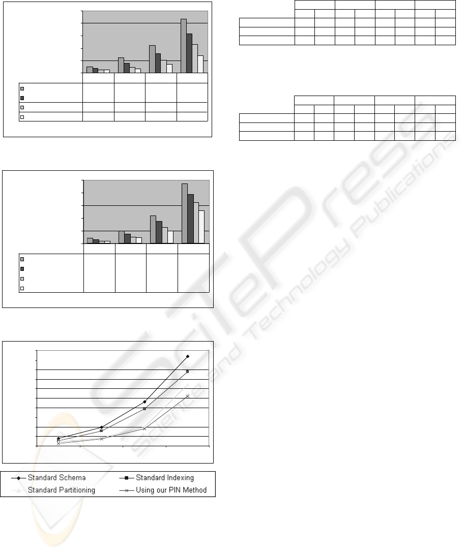
number of simultaneous users increases, showing a

better performance in heavy usage.

700

1400

2100

2800

3500

Simultaneous Users

Time (secon

Standard Schema

326 845 1538 3029

Standard Indexing

264 543 1077 2191

Standard Partitioning

158 306 708 1588

Using our PIN Method

143 237 481 973

1 User 2 Users 4 Users 8 Users

Figure 1: Workload execution time for 1GB TPC-H.

8000

16000

24000

32000

40000

Simultaneous Users

Time (Secon

Standard Schema

3350 7966 17443 37524

Standard Indexing

2463 5725 13621 31038

Standard Partitioning

1458 3670 9854 25653

Using our PIN Method

1427 3386 7918 20745

1 User 2 Users 4 Users 8 Users

Figure 2: Workload execution time for 8GB TPC-H.

4000

8000

12000

16000

20000

24000

28000

32000

36000

40000

1GB 2GB 4GB 8GB

Time (Second

Figure 3: Workload execution for 8 simultaneous users.

Table 5: Performance gain comparison between

techniques in several size TPC-H data warehouses.

1 GB 2 GB 4 GB 8 GB

Methods

Min Max Min Max Min Max Min Max

Standard Index

19% 36% 20% 23% 16% 22% 17% 28%

Standard Partit.

48% 64% 46% 63% 28% 60% 32% 56%

56% 72% 48% 68% 30% 67% 45% 57%

Table 6: Performance gain comparison between

techniques with workload execution by simultaneous

users.

1 User 2 Users 4 Users 8 Users

Methods

Min Max Min Max Min Max Min Max

Standard Index

19% 26% 20% 36% 22% 30% 16% 28%

Standard Partit.

28% 56% 51% 64% 44% 62% 32% 57%

PIN 30% 57% 57% 72% 55% 69% 45% 68%

5 CONCLUSIONS AND FUTURE

WORK

We present an efficient simple and easy to

implement alternative method for optimizing the

performance of data warehouse OLAP queries by

combining partitioning and indexing techniques

based on the existing features of a set of predefined

major SQL data warehouse queries. It also

introduces simple modifications in the database’s

data structures, minimizing the taken up space and

maintenance costs of the data warehouse, in contrast

with other complex partitioning/indexing methods.

The experiments illustrate its efficiency in time

execution and simultaneous user querying, showing

that it overcomes isolated partitioning and indexing

techniques. As future work, we intend to implement

this method in real live data warehouses and

measure its impact on real world system’s

performance.

REFERENCES

Agrawal, S., Chaudhuri, S., Narasayya, V., 2000.

Automated selection of materialized views and

indexes in SQL databases, 26

Int. Conf. on Very

Large Data Bases (VLDB).

Baralis, E., Paraboschi, S., Teniente, E., 1997.

Materialized view selection in a multidimensional

database, 23

Int. Conference on Very Large Data

Bases (VLDB).

Bellatreche, L., Boukhalfa, K., 2005. An Evolutionary

Approach to Schema Partitioning Selection in a Data

Warehouse Environment, Int. Conf. on Data

Warehousing and Knowledge Discovery (DAWAK).

Bellatreche, L., Karlapalem, K., Schneider, M., Mohania,

M., 2000. What can partitioning do for your data

ICEIS 2007 - International Conference on Enterprise Information Systems

176

warehouses and data marts, Int. Database Engineering

and Applications Symposium (IDEAS).

Bellatreche, L., Karlapalem, K., Li, Q., 2000B. Evaluation

of indexing materialized views in data warehousing

environments, Int. Conference on Data Warehousing

and Knowledge Discovery (DAWAK).

Bellatreche, L., Schneider, M., Lorinquer, H., Mohania,

M., 2004. Bringing Together Partitioning,

Materialized Views and Indexes to Optimize

Performance of Relational Data Warehouses, Int.

Conference on. Data Warehousing and Knowledge

Discovery (DAWAK).

Bellatreche, L., Schneider, M., Mohania, M., Bhargava,

B., 2002. PartJoin: an efficient storage and query

execution design strategy for data warehousing, Int.

Conf. on Data W. and Knowledge Discovery

(DAWAK).

Bizarro, P., Madeira, H., 2002. Adding a Performance-

Oriented Perspective to Data Warehouse Design,

International Conference on Data Warehousing and

Knowledge Discovery (DAWAK).

Chaudhuri, S., Narasayya, V., 1997. An efficient cost-

driven index selection tool for Microsoft SQL Server,

Int. Conf. on Very Large Data Bases (VLDB).

Chee-Yong, C., 1999. Indexing techniques in Decision

Support Systems, PhD Thesis, University of

Wisconsin, Madison.

Furtado, P., Costa, J. P., 2002. Time-Interval Sampling for

Improved Estimations in Data Warehouses, Int. Conf.

on Data W. and Knowledge Discovery (DAWAK).

Gupta, H., et al., 1997. Index selection for OLAP, Intern.

Conference on Data Engineering (ICDE).

Gupta, H., Mumick, I. S., 1999. Selection of views to

materialize under a maintenance cost constraint, 8

Int. Conf. Database Theory (ICDT).

Kalnis, P., Papadias, D., 2001. Proxy-server architecture

for OLAP, ACM SIGMOD Int. Conf. on Management

of Data (ICMD).

O’Neil, P., Quass, D., 1997. Improved query performance

with variant indexes, ACM SIGMOD International

Conf. on Management of Data (ICMD).

Sanjay, A., Narasayya, V. R., Yang, B., 2004. Integrating

vertical and horizontal partitioning into automated

physical database design, ACM SIGMOD Int. Conf. on

Management of Data (ICMD).

Transaction Processing Council, TPC Benchmark H,

www.tpc.org

Vassiliadis, P., Sellis, T., 1999. A Survey of Logical

Models for OLAP Databases, ACM SIGMOD Int.

Conf. on Management of Data (ICMD).

PIN: A PARTITIONING & INDEXING OPTIMIZATION METHOD FOR OLAP

177