SOFTWARE COST ESTIMATION USING ARTIFICIAL NEURAL

NETWORKS WITH INPUTS SELECTION

Efi Papatheocharous and Andreas S. Andreou

University of Cyprus, Dept. of Computer Science

75 Kallipoleos str., CY1678 Nicosia, Cyprus

Keywords: Artificial Neural Networks, Software Cost Estimation, Input Sensitivity Analysis.

Abstract: Software development is an intractable, multifaceted process encountering deep, inherent difficulties.

Especially when trying to produce accurate and reliable software cost estimates, these difficulties are

amplified due to the high level of complexity and uniqueness of the software process. This paper addresses

the issue of estimating the cost of software development by identifying the need for countable entities that

affect software cost and using them with artificial neural networks to establish a reliable estimation method.

Input Sensitivity Analysis (ISA) is performed on predictive models of the Desharnais and ISBSG datasets

aiming at identifying any correlation present between important cost parameters at the input level and

development effort (output). The degree to which the input parameters define the evolution of effort is then

investigated and the selected attributes are employed to establish accurate prediction of software cost in the

early phases of the software development life-cycle.

1 INTRODUCTION

Project managers devote extensive effort to achieve

the highest possible control over the software

process and predict, and therefore reduce, the risk

caused by any contingencies. Plans, strategies,

timetables, risk analyses and many other issues are

carefully addressed by project managers in an

attempt to estimate from the beginning of a project

the prospective cost. Especially in the case of

software development, which is considered a very

complex and intractable process affected by various

interrelated parameters, effort and cost are extremely

difficult to predict. Nevertheless, software cost

estimation is identified as a valuable and critical

process. This process includes estimating the size of

the software product to be developed, assessing the

complexity of the functions to be included,

estimating the effort required – usually measured in

person months – developing preliminary project

schedules, and finally, estimating the overall cost of

the project.

In the mid ‘90s, the Standish Group surveyed

over 8000 software projects and the results showed

that for every 100 projects that start there are on

average 94 restarts. Also, an average of 189% of

projects exceed their original cost estimate, their

original time estimate or schedule by 239%, whereas

more than 25% of the projects were completed with

only 25%-49% of the originally-specified features

and functions. In addition, an average of more than

50% of the completed projects had less than 50% of

the original requirements (Standish Group, 1995).

Another survey performed by the Standish Group in

2001 shows that 23% of all software projects are

cancelled before completion, of those projects

completed only 28% are delivered on time, within

budget and with all originally specified features and

the average software project overruns budget by

45% (Laird and Brennan, 2006). In the same year,

the British Computer Society Review revealed that

after surveying 1027 projects, found only 130

successful, and of 500 development projects only 3,

with success being defined as delivering every

functional aspect originally specified, to the quality

agreed on, within the time and costs agreed on

(Coombs, 2003). Reviews on surveys until today

indicate that most projects (60-80%) encounter

effort and schedule overruns (Aggarwal et al., 2005).

The above statistics reveal and underline the

inherent problems the software process faces and

justify the difficulties observed with project

management activities.

398

Papatheocharous E. and S. Andreou A. (2007).

SOFTWARE COST ESTIMATION USING ARTIFICIAL NEURAL NETWORKS WITH INPUTS SELECTION.

In Proceedings of the Ninth International Conference on Enterprise Information Systems - DISI, pages 398-407

DOI: 10.5220/0002380803980407

 SciTePress

The accurate and reliable software cost

prediction can significantly increase the productivity

of an organisation and can facilitate the decision

making process (Briand et al., 1999), while, at the

same time, it is highly important to both developers

and customers (Leung and Fan, 2002). Project

managers commonly stress the importance of

improving estimation accuracy and the need for

methods to support better estimates, as these can

help diminish the problems concerning the software

development process and contribute to better project

planning, tracking and control, thus paving the way

for successful project delivery (Lederer and Prasad,

1992). Once a satisfactory and reliable software cost

model is devised, it can then be used for efficiently

developing software applications in an increasingly

competitive and complex environment. The model

may thus constitute the basis for contract

negotiations, project charging, classification of tasks

and allocation of human resources, task progress

control, monitoring of personnel and other resources

according to the time schedule, etc.

The parameters anticipated to affect software

development cost are not easy to define, are highly

ambiguous and difficult to measure particularly at

the early project stages. The hypothesis here is that

if we manage to detect those project characteristics

that decisively influence the evolution of software

cost and assess their impact then we may provide

accurate estimations. Therefore, finding the

fundamental characteristics of the software process

is critical, as these can lead to the creation of various

computational models that aim at measuring or

predicting certain factors affecting this process, such

as software development effort, quality and

productivity. The work presented in this paper aims

to provide accurate predictions of software

development cost by utilising computational

intelligent methods along with Input Sensitivity

Analysis (ISA) to find the optimal set of input

parameters that seem to describe better the cost of a

software project, especially in early phases of the

software development life-cycle (SDLC).

The rest of the paper is organised as follows:

Section 2 presents a brief overview of the relevant

software cost estimation literature and outlines the

basic concepts of artificial neural networks, the latter

constituting the basis of our modelling attempt.

Section 3 introduces the dataseries used for

experimentation and describes in detail the cost

estimation methodology suggested. Section 4

provides the application of the methodology and

discusses the experimental results obtained,

commenting on the factors that mostly affect

software cost. Finally, Section 5 draws the

concluding remarks and suggests future research

steps.

2 COST ESTIMATION MODELS:

A THEORETIC BACKGROUND

During the end of the 50s and 60s, researchers and

software engineers began focusing on software cost

estimation. Since then various estimation techniques

and models have been proposed in order to achieve a

better and more accurate cost prediction. Software

cost estimation is conceived in this paper as the

process of predicting the amount of effort required

to develop software. The success of this process lies

with the quality of the data and the selected

parameters used for performing the estimation.

A considerable amount of the models used for

software cost estimation are either cost-oriented,

providing direct estimates of effort, or constraint

models, expressing the relationship between the

parameters affecting effort over time. COCOMO

(Constructive Cost Model), an example of a cost

model, has a primary cost factor (size) and a number

of secondary adjustment factors or cost drivers

affecting productivity. Since its first publication

(Boehm, 1981) it has been revised to newer versions

called COCOMO II (Boehm et al., 1995) and later in

(Boehm, 1997), mixing three cost models, each

corresponding to a stage in the software life-cycle:

Applications Composition, Early Design, and Post

Architecture, appearing to be more useful for a

wider collection of techniques and technologies.

SLIM (Software Life-cycle Model), an example

of a constraint model, is applied on large projects,

exceeding 70000 lines of code and assumes that

effort for software projects is distributed similarly to

a collection of Rayleigh curves (Putnam and Myers,

1992). It supports most of the popular size

estimating methods including ballpark techniques,

function points (Boehm et al., 2000), component

mapping, GUI (object) sizing, sizing by module etc.

(visit the Quantitative Software Management

website: http://www.qsm.com, for more information

on recently developed SLIM tools). A stepwise

approach, utilising software and manpower build-up

equations, is used and the necessary parameters that

must be known upfront for the model to be

applicable are the system size, the manpower

acceleration and the technology factor.

Software cost models are evaluated considering

certain error criteria, with the most common method

comparing the estimated with the actual effort.

Existing software cost models experience

SOFTWARE COST ESTIMATION USING ARTIFICIAL NEURAL NETWORKS WITH INPUTS SELECTION

399

fundamental problems based on the criteria results,

especially if we consider the suggestion that a model

is acceptable if 75% of the predicted values fall

within 25% of their actual values (Fenton, 1997).

The difficulty lies with specifying which metrics to

use as inputs in a cost model and obtaining sample

values rated with high quality in terms of reliability,

objectivity and homogeneity (MacDonell and Gray,

1997). Unfortunately, in most of the models there is

not an agreement on which parameters to use to

provide better estimates. Since for many metrics the

actual value is never known with certainty before the

project is completed, they are often given values that

managers or experts anticipate, or may be created

using past project data samples. While the former

case suffers from subjectivity, in the latter case the

difficulty in having metric values increases as there

is lack of publicly available, reliable and

homogenous data. Homogenous project data sets

may become available only if they are carefully

collected, under the same conditions (similar

processes, technologies, environments, people and

requirements) and as long as a consistent measuring

mechanism is used. In addition, collaboration

between the industry and research institutions is

relatively narrowed and confined only to certain

parts of the world, while at the same time historical

databases of cost measurements are limited and

scattered due to the difficult, costly and time-

consuming nature of the data gathering procedure.

While various studies attempted to predict

development effort, results reported indicate high

dependence on data and input parameters. In

MacDonell and Gray (1997) Artificial Neural

Networks (ANN) and Fuzzy Models were used on

the Desharnais dataset. The performance of the

ANN (measured using the Correlation Coefficient

(CC) and the Mean Relative Error (MRE) measures)

was not overly impressive, with 7 out of the 27

validation cases not being predicted even within

50%, while the best result obtained marked

CC=0.7745 and MRE=0.4586. Idri et al. (2002)

attempted to estimate software cost using

backpropagation trained Multi Layer Perceptrons

(MLP) on the COCOMO ’81 dataset and their best

results reached MREs equal to 1.5%, 203.66%,

84.35%, while the main conclusion was that

accuracy increases as the number of projects in the

training process rises. In Finnie and Wittig (1997) , a

back-propagation trained MLP was used on the

Desharnais and ASMA datasets presenting

encouraging results, with MRE=27% and

MRE=17% respectively. Jeffery et al. (2000)

compared three estimation techniques, Ordinary

least-squares (OLS) Regression and analogical and

algorithmic cost estimation on company-specific

(Megatec) and multi-organisational (ISBSG) data

and the results showed Median MRE=0.38,

pred(0.25)=0.21 and Median MRE=0.66 and

pred(0.25)=0.05 respectively. The need for

qualitative and consistent datasets is revealed once

again as the estimations produced using data

measured in the same development environment

(Megatec) seem more accurate than with scattered

information (ISBSG). Recently, efforts have been

made to extract and analyse a subset of important

variables to provide more effective and complete

analysis in terms of both quality and quantity

(Santillo et al., 2005).

Summarising the above, the use of computational

intelligent techniques for software cost estimation is

quite rich. Nevertheless, the results obtained thus far

are not satisfactory, and, moreover, not consistent in

terms of prediction accuracy and type of cost factors

used in the models. In this work we attempt to cover

this gap and achieve on one hand high cost

prediction accuracy and on the other propose a

systematic way to select the most appropriate cost

factors in the context of ANN. ANN consist of

interconnected nodes able to deal with complex

domains, perform intelligent computations and are

utilised for forecasting sample data to generalise

knowledge learned through examples without

requiring an a priori mathematical expression of the

output in terms of the inputs used. Further details

may be found in (Haykin, 1999).

3 DATA AND METHODOLOGY

We move now to describing firstly the available

datasets and the necessary pre-processing activities,

and secondly our methodology for identifying the

most critical factors within the datasets which

determine software cost through the application of

sensitivity analysis on selected ANN.

3.1 Description of Datasets

The Desharnais dataset (Desharnais, 1988) includes

observations for more than 80 systems developed by

a Canadian software development house at the end

of 1980 and describes 9 features. The basic

characteristics of the Desharnais dataset account for

the following: project name, development effort

measured in hours, team’s experience, project

manager’s experience, both measured in years,

number of transactions processed, number of

entities, unadjusted and adjusted Function Points,

ICEIS 2007 - International Conference on Enterprise Information Systems

400

length of development, scale of the project and

development language.

The second dataset called ISBSG (International

Software Benchmarking Standards Group;

Repository Data Release 9) contains an analysis of

software costs for a group of projects. The projects

come from a broad cross section of industry and

range in size, effort, platform, language and

development technique data. These projects undergo

a series of quality checks for completeness and

integrity and then they are rated in order to achieve

the grade of usefulness of the data for various

analyses. The ISBSG reports that this dataset

represents the more productive projects in the

industry, rather than industry norms, because

organisations are considered to be among the best

software development houses and also, they may

have chosen to submit only their best projects rather

than typical ones. Therefore, the projects have not

been selected randomly and the dataset most

probably is subject to biases. The main issue that is

being raised here is the homogeneity of the

dataseries which stems by the fact that the recorded

projects come from different companies all over the

world. Therefore, the variety in people, processes,

practices, tools, etc. suggest that there is significant

heterogeneity in fundamental parameters affecting

the measurements.

3.2 Data Pre-processing

The aforementioned datasets were used in a stepwise

approach aiming firstly either to limit the number of

inputs used for software development cost

estimation, or define the relationship among certain

parameters affecting effort over time; secondly, to

provide better accuracy to software cost prediction.

The process suggested in this paper for achieving the

above, begins with data pre-processing, performed

on the initial dataseries in order to prepare them for

the next steps. The data pre-processing included the

subtraction of projects with null values in the

attributes from the two datasets, whereas from the

ISBSG dataset we also subtracted certain parameters

with incomplete data, or alphanumeric data

(containing categorical variables instead of

numerical) or parameters with no direct or apparent

affect on software cost. After data sampling, we

chose representative subsets from the whole

populations, 78 projects and available attributes (10

in number as described before) for the Desharnais

dataset and 739 projects and 19 attributes for the

ISBSG dataset. The latter attributes are: project

name, functional size (A1), adjusted function points

(A2), reported PDR (afp) (A3), project PDR (ufp)

(A4), normalized PDR (afp) (A5), normalized PDR

(ufp) (A6), project elapsed time (A7), project

inactive time (A8), resource level (A9), input count

(A10), output count (A11), enquiry count (A12), file

count (A13), interface count (A14), added count

(A15), changed count (A16) and deleted count

(A17). Additionally, normalization in the range [-1,

1] was performed on the data since learning was

based on the gradient descent with momentum

weight / bias learning function which works with

neuron transfer functions operating in this value

range. Thus, normalization on the data would

prevent the loss of information encapsulated in

values with small numerical differences.

3.3 Neural Networks and Data Input

Sensitivity Analysis

As previously mentioned, our methodology utilises

ISA performed on ANN to define which attributes

from the available datasets mostly affect and

ultimately define the value of software cost. The

main argument here is that software cost analysis

methods and models would be safer if we can isolate

the important underlying parameters more likely to

cause critical cost differences from the metrics

population in the datasets. The importance of the

project attributes is measured via sensitivity analysis

and more specifically by the input weights

associated in each network created and trained,

provided that the network yielded high prediction

ability. The latter is assessed using specific error

metrics that compare the actual sample values to the

predictions outputted by the network. Sensitivity

analysis is a good method to assure that results are

robust, ensure that the relationship and influence

among factors and cost are comprehended correctly

and remove outlying parameters from the model. As

also pointed out by Saltelli (2004) sensitivity

analysis’ scope should be specified beforehand. In

our case we use ANN and then perform sensitivity

analysis on their inputs describing software cost data

to identify the relevant factors and their degree of

dependence with the output factor which is effort. In

this way, we attempt to simplify the model and

prioritise factors in an order of importance so as to

guide further research and future software cost

estimations. Our main effort is centralised on

whether we can minimise the number of factors used

for cost prediction to only those factors that can be

evaluated from the early software development

cycle, having relatively easier, lower cost and time

data gathering processes and also ensuring as

accurate cost estimates as possible.

SOFTWARE COST ESTIMATION USING ARTIFICIAL NEURAL NETWORKS WITH INPUTS SELECTION

401

3.4 Design of the Experiments

The core architecture utilised in our experiments

consists of a feed-forward MLP network, with a

single hidden layer. Several network topologies are

created comprising different number of hidden

neurons: We start with networks having the number

of hidden neurons (NHN) equal to the number of

inputs (NI) and we proceed producing new ANN

architectures by increasing HN by one until it

doubles NHN. Each network is trained to learn and

predict the behaviour of the available datasets and

characterise the relationship among the inputs and

the output, the latter being the development effort.

The data is divided into training, validation and

testing sets. The training set is used during the

learning process, the validation set is used to ensure

that no overfitting occurs in the final result and that

the network was able to generalise the knowledge

gained. The testing set is an independent dataset, i.e.,

does not participate during the learning process and

measures how well the network performs with

unknown data. The extraction is made randomly

with 70% of the data samples used for training, 20%

for validation and 10% for testing. During training

the inputs are presented to the network in patterns

(inputs/output) and corrections are made on the

weights of the network according to the overall error

in the output and the contribution of each node to

this error. After training we take the best 20% of our

ANN in terms of accuracy and apply the ISA as an

extension to the whole process, according to which

the weights of each input to the hidden layer are

summed up, thus developing an order of significance

for the input parameters. The higher the sum of

weights for a certain parameter is the highest the

contribution of that parameter in defining the final

output of the network. Using this significance values

we move to filtering parameters, i.e. some of the

inputs are accepted as important software cost

factors while others are rejected, according to two

different criteria: a Strict (S) and a Less Strict (LS)

method. Each method identifies as significant those

inputs for each network whose sum of weights is

above a certain threshold. The threshold for the strict

method is defined in equation (1), while that the less

strict method in equation (2).

)min()max(

11 nn

wwww

−

(1)

25,0)max(

∗−=

www

(2)

The threshold for the strict method is specified as

such to consider significant those inputs whose sum

of weights is higher than half the difference between

the corresponding maximum and minimum weight

sums among the inputs of the network. Whereas, the

threshold for the less strict method is more flexible,

characterizing as significant those inputs whose

summed weights value is higher than the 25% of the

corresponding ANN’s maximum value. The final

criterion to decide which inputs to keep and perform

new experiments (final runs) is equation (3).

___

ANNsnumbertotal

WANNsofnum

totalrate

LSorS

ith

(3)

Equation (3) simply calculates for each input

parameter i the percentage to which it was rated

significant using each method (S or LS) Therefore,

we practically enhance the specified thresholds with

a second criterion, i.e., the input should appear as

important parameter in more than half of the best

ANN trained. In this way, not only the weights

define which inputs to accept as important factors to

cost estimation, but also whether these variables are

also considered important to more than half of the

best ANN is investigated for enhancing the

assessment of their overall significance.

Using the results obtained according to equation

(3) the inputs considered more significant and thus

safer to use for software cost prediction are isolated

for including them in the final set of experiments;

we will call this the Final Parameters (FP) set. It

should be noted at this point that the whole process

(starting from ANN creation and training and ending

to the formation of the FP set) is repeated 10 times,

each time picking randomly the order of the projects

from the datasets. This accounts for the random and

heuristic nature of ANN and yields more reliable,

robust and unbiased results. The leading variables

for the final runs are selected according to how

many times during the experiments they were

selected as important by both the ISA and the S and

LS threshold, i.e., how many times they were

present in the FP sets of the 10 repetitions.

4 EXPERIMENTAL RESULTS

The performance of the ANN is evaluated using the

following error metrics:

)(

)()(

)(

ixix

nRMAE

act

predact

∑

−

(4)

(

) ()

[

]

()()

⎥

⎦

⎤

⎢

⎣

⎡

−

⎥

⎦

⎤

⎢

⎣

⎡

−

−−−

∑∑

∑

npred

pred

nact

act

npred

pred

nact

act

xixxix

)()(

(5)

[]

)(

)()(

)(

∑

−

act

xix

nRMSEnRMSE

nNRMSE

(6)

ICEIS 2007 - International Conference on Enterprise Information Systems

402

where

[]

∑

−=

actpred

ixix

nRMSE

)()(

)(

(7)

lpred =)(

(8)

In equations (4) to (8) x

act

represents the actual

value of the data sample and x

pred

the predicted one.

The Relative Mean Absolute Error (RMAE) given

by (4) shows prediction error by focusing on the

actual sample being predicted (normalization). The

Correlation Coefficient (CC) between the actual and

predicted series, given by (5), measures the ability of

the predicted samples to follow the upwards or

downwards of the original series. An absolute CC

value equal or near 1 is interpreted as a perfect

follow up of the original series by the forecasted

one. A negative CC sign indicates that the

forecasting series follows the same direction of the

original with negative mirroring, that is, with 180

rotation about the time-axis.

The Normalized Root Mean Squared Error

(NRMSE) detects the quality of predictions: if

NRMSE=0 then prediction is perfect; if NRMSE=1

then prediction is no better than taking the mean of

the actual values as the predicted one.

Equation (8) defines how many data predictions k

out of n (total number of data points predicted)

performed well, i.e., their RE metric given in

equation (9) is lower than level l. In our experiments

the parameter l was set equal to 0.25.

)(

)()(

)(

ixix

nRE

act

predact

−

(9)

Additionally, the well known error metrics Mean

Square Error (MSE) and Mean Absolute Error

(MAE) were used to evaluate the ANN’s

performance. Although both metrics suffer from

scaling dependence, their results will be reported in

this paper, as well so as to make comparisons with

relevant work feasible.

In Table 1 we summarise the results from the

best ANN in one of the ten iterative experiments

performed with the Desharnais dataset, reporting the

training and testing errors, while Table 2 shows the

corresponding results with the ISBSG dataset. In the

middle part of these tables we present the average

weights of the input parameters and at the lower part

the leading inputs for cost estimation are indicated

by each of the two thresholds (S and LS).

Commenting on the results of both tables, based

on the error figures we can observe a very successful

modelling and forecasting of development effort

data samples as the RMAE and NRMSE values are

quite low, while CC and pred(l) are more than

adequately high. These findings indicate accurate

predictions of software cost based on historical data

of the selected input parameters.

The ISA performed on the networks suggested a

first order of significance for the inputs (average

weights of 10 repetitions). This significance was

then refined using the S and LS approaches which

indicated the important parameters (marks on

tables). These indications were combined with

equation (3) and the important parameters marked in

more than 50% of the best networks (in our case

having more than 2 marks) were selected for the

final experiments (FP set).

The final runs included the training and testing of

a feed-forward MLP network, with a single hidden

layer comprising once again a varying number of

neurons and using the inputs included in the FP set

resulted from the S approach and the LS approach.

Additionally a third approach was followed based on

which we used as inputs those parameters that

appeared more frequently in the results of the ISA

alone and can be measured during the early

development phases. With the latter approach (called

“ideal”) we attempt to minimise the prediction

complexity by diminishing its dependence on many

factors which are difficult to measure at the early

project stages and increase the time and cost

overheads of the measuring procedure.

Tables 3 and 4 list the results of the best

performed ANN conducted for the Desharnais and

ISBSG datasets respectively using the FP parameters

set and the ideal approach. More specifically, the

inputs used for the final runs with the Desharnais

dataset as suggested by the S approach were Points

Adjusted and Points Non Adjusted, while those of

the LS approach were Team Experience,

Transactions, Points Adjusted, Envergure and Points

Non Adjusted. The “ideal” approach for early phase

estimation used Team Experience, Manager

Experience, Points Adjusted and Points Non

Adjusted. The FP set for Desharnais appears

consistent in creating a strong relationship among

work effort and software size measured with

function points. The inputs used for the final runs of

the ISBSG dataset as suggested by the S approach

were the Normalised PDR (afp), File count and the

Added count, while the LS approach suggested

Normalised PDR (afp), Enquiry count, File count,

Added count, Changed count as the important ones

The “ideal” estimation used as inputs the Functional

Size, the Adjusted Function points and the

Normalised PDR (afp). One may observe here the

following: (i) predictions of the effort in both

datasets are equally successful as with the original

experiments with the whole spectrum of the

SOFTWARE COST ESTIMATION USING ARTIFICIAL NEURAL NETWORKS WITH INPUTS SELECTION

403

Table 1: Desharnais dataset ANN Experimental Results.

ANN Experimental Results / Training And Testing Errors (Indicative runs – out of 10 iterations)

TRAINING TESTING

ANN.

NRMSE CC MSE RMAE MAE pred(l) NRMSE CC MSE RMAE MAE pred(l)

9-20-

0.2328 0.9720 0.0058 0.1012 0.0592 0.9811 0.3289 0.9552 0.0026 0.0470 0.0366 1

9-16-

0.2489 0.9682 0.0066 0.1033 0.0597 1 0.3666 0.9325 0.0033 0.0610 0.0440 1

9-10-

0.3055 0.9514 0.0100 0.1235 0.0729 0.9811 0.3777 0.9215 0.0035 0.0634 0.0504 1

9-19-

0.1797 0.9834 0.0034 0.0709 0.0453 1 0.4661 0.8997 0.0053 0.0735 0.0600 1

ANN Experimental Results / Average Weights for each Input

ANN Team Exp. Manager Exp. Length Transactions Entities Points adj. Envergure Points non adj. Language

9-20-

0.0658 0.0910 0.0238 0.0606 0.2068 0.0790 0.0577 0.1495 0.0658

9-16-

0.1232 0.0109 0.0354 0.2124 0.0633 0.4583 0.0290 0.0300 0.1232

9-10-

0.1096 0.1718 0.0699 0.0845 0.2855 0.3958 0.0698 0.1939 0.1096

9-19-

0.0855 0.0176 0.1947 0.0951 0.2519 0.1112 0.1179 0.0312 0.0855

ANN Experimental Results Input Sensitivity Analysis / Strict (S) and Less Strict (LS) Approach

Team Exp. Manager Exp. Length Transactions Entities Points adj. Envergure Points non adj. Language

ANN

S LS S LS S LS S LS S LS S LS S LS S LS S LS

9-20-1 9 9 9 9 9 9 9 9 9

9-16-1 9 9 9 9 9

9-10-1 9 9 9 9 9 9 9 9

9-19-1 9 9 9 9 9 9 9 9

Table 2: ISBSG dataset ANN Experimental Results.

ANN Experimental Results / Training And Testing Errors (Indicative runs – out of 10 iterations)

TRAINING TESTING

ANN

NRM

CC MSE RMAE MAE pred(l) NRMSE CC MSE RMAE MAE pred(l)

18-22-1

0.385

0.9237 0.0020 0.0349 0.0294 1 0.3761 0.9381 0.0044 0.0642 0.0474 1

18-23-1

0.430

0.9026 0.0026 0.0355 0.029 0.9980 0.3764 0.9509 0.0048 0.0541 0.0430 0.9932

18-35-1

0.493

0.8727 0.0034 0.0434 0.0373 0.9980 0.3587 0.9482 0.0044 0.0532 0.0432 0.9932

18-19-1

0.329

0.9452 0.0015 0.0300 0.0256 1 0.2616 0.9675 0.0025 0.0409 0.0328 1

ANN Experimental Results / Average Weights for each Input

NHN

A1 A2 A3 A4 A5 A6 A7 A8 A9 A10 A11 A12 A13 A14 A15 A16

0.1

0.0

0.10 0.02 0.086 0.01 0.06 0.03 0.05 0.05 0.014 0.14 0.056 0.016 0.11 0.05

0.0

0.09 0.18 0.153 0.13 0.02 0.01 0.03 0.05 0.009 0.07 0.010 0.131 0.06 0.04

0.0

0.04 0.03 0.013 0.01 0.05 0.10 0.13 0.08 0.128 0.06 0.075 0.088 0.11 0.05

0.0

0.1

0.00 0.15 0.185 0.18 0.09 0.03 0.05 0.11 0.027 0.18 0.079 0.011 0.15 0.01

ANN Experimental Results Input Sensitivity Analysis / Strict (S) and Less Strict (LS) Approach

A1 A2 A3 A4 A5 A6 A7 A8 A9 A10 A11 A12 A13 A14 A15 A16 A17

9 9 9 9 9 9 9 9 9 9 9 9 9 9 9 9 9 9

9 9 9 9 9 9 9 9 9 9 9 9 9 9 9 9

9 9 9 9 9 9 9 9 9 9 9 9 9 9 9 9 9 9 9 9

* NHN denotes the number of hidden neurons in the ANN topology at the upper part of the table

ICEIS 2007 - International Conference on Enterprise Information Systems

404

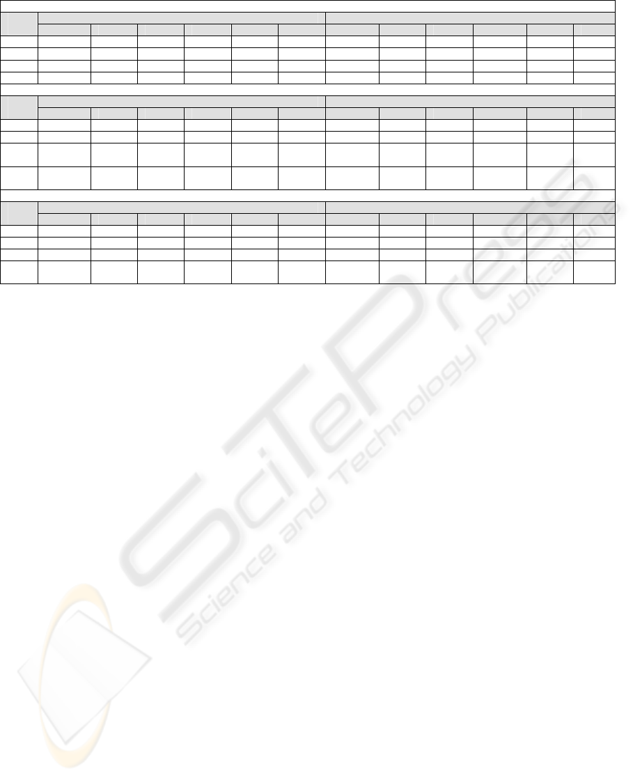
Table 3: Desharnais dataset ANN Final Runs.

Strict (S) Approach

TRAINING TESTING ANN

Arch.

NRMSE CC MSE RMAE MAE pred(l) NRMSE CC MSE RMAE MAE pred(l)

2-3-1 0.8147 0.5697 0.0608 0.6006 0.1807 0.9245 0.6916 0.6999 0.0169 0.1956 0.0907 1

2-4-1 0.8254 0.5621 0.0624 0.6018 0.1878 0.9245 0.7172 0.6762 0.0181 0.2089 0.1027 1

2-5-1 0.8413 0.5490 0.0648 0.6276 0.1980 0.9245 0.8602 0.5801 0.0261 0.2431 0.1125 1

2-6-1 0.7892 0.6044 0.0570 0.5872 0.1762 0.9245 0.7202 0.6759 0.0183 0.2026 0.0905 1

Less Strict (LS) Approach

TRAINING TESTING ANN

Arch.

NRMSE CC MSE RMAE MAE pred(l) NRMSE CC MSE RMAE MAE pred(l)

5-7-1 0.7008 0.7111 0.0449 0.4937 0.1554 0.9245 0.6550 0.8330 0.0151 0.1844 0.0806 1

5-8-1 0.6155 0.7846 0.0347 0.3681 0.1298 0.9434 0.6967 0.7719 0.0171 0.1875 0.0767 1

5-11-

0.6742 0.7338 0.0416 0.4528 0.1603 0.9245 0.6104 0.8410 0.0131 0.1718 0.0826 1

5-12-

0.7655 0.6350 0.0536 0.5377 0.1649 0.9245 0.6414 0.8040 0.0145 0.1780 0.0781 1

“Ideal” (Early Phase) Approach

TRAINING TESTING ANN

Arch.

NRMSE CC MSE RMAE MAE pred(l) NRMSE CC MSE RMAE MAE pred(l)

4-6-1 0.8767 0.4702 0.0704 0.7095 0.1987 0.9245 0.8772 0.4852 0.0272 0.2463 0.1108 1

4-7-1 0.7294 0.6769 0.0487 0.6134 0.1637 0.9245 0.7052 0.7405 0.0175 0.2044 0.0932 1

4-8-1 0.7556 0.6466 0.0523 0.5851 0.1755 0.9245 0.7419 0.6769 0.0194 0.2095 0.0945 1

4-10-

0.8014 0.5885 0.0588 0.5983 0.1819 0.9245 0.8390 0.5076 0.0248 0.2370 0.1349 1

whole spectrum of the available parameters

acting as inputs, something which leads to infer that

we actually managed to identify those parameters

that describe best the cost in terms of ANN learning,

(ii) the “ideal” case is also quite successful, although

a very small and in some cases negligible prediction

accuracy degradation may be observed, a fact that

leads us to conclude that if we are confined to those

variables that can indeed be measured early we can

produce accurate cost estimations.

Overall, the results appear to be more than

promising indicating high predictive power, good

estimates and very low error rates with the use of

ANN. With the use of the FP set, after the ISA, the

error rates appear slightly worse but this is

considered minimal trade-off since we managed to

minimise the number of the contributing factors to

software cost. The approach resulted in slight

deterioration in terms of predictive power;

nevertheless, it was able to disengage the cost

estimation process from the difficult and time-

consuming process of gathering values for a large

variety of metrics, something which enables the

production of cost estimations from the first phases

of the project using cost factors that are available

early in the development process. The stepwise

approach we proposed resulted in devising a

satisfactory and reliable software cost model that can

be afterwards used as a basis for efficiently

assessing software development cost.

4 CONCLUSIONS

This work proposed a stepwise process that utilises

Artificial Neural Networks (ANN) and Input

Sensitivity Analysis (ISA) to create a software cost

prediction model based on historical samples.

Firstly, different topologies of ANN were trained

with the Desharnais and ISBSG datasets and then

ISA was applied on the best performed networks to

calculate the weights of each input parameter fed

using a Strict (S) and a Less Strict (LS) threshold

approach. This led to the definition of the significant

inputs that determine the course of estimating

development cost. We observed a relative

consistency in the selected parameters by each

approach, with inputs such as the Points Adjusted

for the Desharnais and the Normalised PDR (afp) for

the ISBSG being universally considered as

important cost drivers in all experiments conducted.

Finally, the significant parameters were isolated

and used separately for new experiments The

performance of the model was assessed through

various error measures, with the results indicating

highly accurate effort estimates. Therefore, we

achieved to minimise the number of parameters used

for software cost prediction and concluded that only

an average of 3 to 5 specific parameters is enough to

provide good effort estimates.. Moreover, we

succeeded in identifying a small set of parameters,

which can be measured early in the software life

cycle, that result in equally successful estimates as

with using all the available input parameters.

SOFTWARE COST ESTIMATION USING ARTIFICIAL NEURAL NETWORKS WITH INPUTS SELECTION

405

Table 4: ISBSG dataset ANN Final Runs.

Strict (S) Approach

TRAINING TESTING ANN

Arch.

NRMS

CC MSE RMAE MAE pred(l) NRMSE CC MSE RMAE MAE pred(

3-4-1 0.6982 0.7227 0.0059 0.0464 0.0399 0.9980 0.5246 0.8523 0.0077 0.0374 0.0350 0.99

3-5-1 0.5063 0.8621 0.0031 0.0382 0.0322 1 0.2195 0.9766 0.0013 0.0260 0.0242 1

3-6-1 0.6783 0.7378 0.0055 0.0499 0.0425 0.9980 0.4290 0.9086 0.0052 0.0418 0.0390 0.99

3-7-1 0.6342 0.7749 0.0048 0.049 0.0419 1 0.3564 0.9386 0.0035 0.0390 0.0360 1

Less Strict (LS) Approach

TRAINING TESTING ANN

Arch.

NRMS

CC MSE RMAE MAE pred(l) NRMSE CC MSE RMAE MAE pred(

5-6-1 0.5721 0.8243 0.0039 0.0462 0.0394 1 0.3031 0.9565 0.0026 0.0384 0.0355 1

5-7-1 0.6942 0.7251 0.0058 0.0499 0.0427 0.9980 0.5229 0.8617 0.0077 0.0445 0.0418 0.99

5-11-

0.6718 0.7402 0.0054 0.0400 0.0343 0.9980 0.5984 0.8055 0.0101 0.0389 0.0360 0.99

5-12-

0.8378 0.5570 0.0085 0.0563 0.0482 0.9980 0.6938 0.7178 0.0136 0.0495 0.0457 0.99

“Ideal” (Early Phase) Approach

TRAINING TESTING ANN

Arch.

NRMS

CC MSE RMAE MAE pred(l) NRMSE CC MSE RMAE MAE pred(

4-6-1 0.6151 0.7880 0.0045 0.0495 0.0419 1 0.2968 0.9559 0.0024 0.0392 0.0363 1

4-7-1 0.4826 0.8755 0.0028 0.0333 0.0280 1 0.2355 0.9731 0.0015 0.0258 0.0239 1

4-8-1 0.3924 0.9197 0.0018 0.0293 0.0250 1 0.1962 0.9805 0.0010 0.0232 0.0218 1

4-9-1 0.4774 0.8785 0.0027 0.0323 0.0270 1 0.2805 0.9602 0.0022 0.0276 0.0257 1

The overall benefit of our approach is a faster, less

complex and accurate cost estimation model, even

from the early development phases, which, among a

variety of well known and used parameters, traces

and addresses only those factors that decisively

influence the evolution of software cost.

Future work will include further investigation of

the proposed approach focusing on the use of other

datasets and examining the consistency of the

significant cost factors derived. Our goal is to

incorporate in our model enterprise or organization

dependent factors and assess the degree to which a

set of inputs measured under the same software

development conditions, team and project

characteristics, may be used for real situation

software cost estimation. Furthermore, the results

derived from the “ideal” scenario allow the reuse of

this knowledge in estimating cost for a small-to-

medium software enterprises usually working on

projects of similar size and scale. Finally, we plan to

conduct experiments on the basis of a more

systematic approach, utilising evolutionary methods,

such as Genetic Algorithms, to evolve ANN

topologies and improve their predictive power for

producing reliable cost estimates.

REFERENCES

Aggarwal, K., Singh, Y., Chandra, P. and Puri, M., 2005.

Bayesian Regularization in a Neural Network Model

to Estimate Lines of Code Using Function Points.

Journal of Computer Sciences 1 (4), pp. 504-508.

Boehm, B.W., 1981. Software Engineering Economics.

Prentice Hall.

Boehm, B.W., Abts, C., and Chulani, S., 2000. Software

development cost estimation approaches – A survey.

In Annals of Software Engineering 10, p. 177-205.

Boehm, B.W., Abts, C., Clark, B., and Devnani-Chulani.

S., 1997. COCOMO II Model Definition Manual. The

University of Southern California.

Boehm, B.W., Clark B., Horowitz E. and Westland C.,

1995. Cost Models for Future Software Life Cycle

Processes: COCOMO 2.0. Annals of Software

Engineering, Vol. 1, pp. 57-94.

Briand, L. C., Emam K. E., Surmann D., Wieczorek I.,

Maxwell K., 1999. An Assessment and Comparison of

Common Software Cost Estimation Modeling

Techniques. Proceedings International Conference

Software Engineering, pp. 313-322.

Coombs, P., 2003. IT Project Estimation: A Practical

Guide to the Costing of Software, Cambridge

University Press.

Desharnais, J. M., 1988. Analyse Statistique de la

Productivite des Projects de Development en

Informatique a Partir de la Technique de Points de

Fonction. Université du Québec: MSc. Thesis,

Montréal.

ICEIS 2007 - International Conference on Enterprise Information Systems

406

Fenton, N.E. and Pfleeger, S.L., 1997. Software Metrics: A

Rigorous and Practical Approach. International

Thomson Computer Press.

Finnie, G. R., Wittig G. E. and Desharnais J. M., 1997. A

comparison of software effort estimation techniques

using function points with neural networks, case based

reasoning and regression models. J. of Systems

Software, Vol. 39, pp. 281-89.

Haykin, S., 1999. Neural Networks: A Comprehensive

Foundation, Prentice Hall.

Idri, A., Khoshgoftaar T. M. and Abran A., 2002. Can

Neural Networks be easily interpreted in Software

Cost Estimation? In Proc. of the 2002 IEEE Intern.

International Software Benchmarking Standards Group,

Repository Data Release 9,t

Jeffery, R., Ruhe M. and Wieczorek I., 2000. A

comparative study of two software development cost

modeling techniques using multi-organizational and

company-specific data. Information and Software

Technology, Vol. 42, No. 14, pp. 1009-1016.

Laird, L. M. and Brennan, M. C., 2006. Software

Measurement and Estimation: A Practical Approach.

John Wiley & Sons, Inc.

Lederer, A. L. and Prasad J., 1992. Nine management

guidelines for better cost estimating. Comm. of the

ACM, Vol. 35, No. 2, pp. 51-59.

Leung, H. and Fan Z., 2002. Software Cost Estimation. In

Handbook of Software Engineering and Knowledge

Engineering, Vol. 2, World Scientific.

MacDonell S. G. and Gray A. R., 1997. Applications of

Fuzzy Logic to Software Metric Models for

Development Effort Estimation. Proc. of 1997:

Annual Meeting of the North American Fuzzy

Information Processing Society – NAFIPS, Syracuse

NY, USA, IEEE, pp. 394-399.

Putnam, L. H. and Myers W., 1992. Measures for

Excellence, Reliable Software on Time, Within Budget.

Yourdan Press, Englewood Cliffs N.J.

Saltelli, A., 2004. Global Sensitivity Analysis: An

Introduction. In Proc. 4th Intern. Conf. on Sensitivity

Analysis of Model Output (SAMO ’04), pp. 27-43.

Santillo, L., Lombardi, S. and Natale D., 2005. Advances

in statistical analysis from the ISBSG benchmarking

database. Proceedings of SMEF, pp.39-48.

The Standish Group, CHAOS Chronicles, Standish Group

Internal Report, 1995, Available at

<http://www.standishgroup.com/>.

SOFTWARE COST ESTIMATION USING ARTIFICIAL NEURAL NETWORKS WITH INPUTS SELECTION

407