FEEDFORWARD NEURAL NETWOTKS WITHOUT

ORTHONORMALIZATION

∗

Lei Chen, Hung Keng Pung and Fei Long

Network Systems and Service Lab., Department of Computer Science, National University of Singapore, Singapore

Keywords:

Feedforward neural networks, kernel function, orthonormal transformation, Extreme Learning Ma-

chine(ELM), approximation, generalization performance.

Abstract:

Feedforward neural networks have attracted considerable attention in many ﬁelds mainly due to their approx-

imation capability. Recently, an effective noniterative technique has been proposed by Kaminski and Stru-

millo(Kaminski and Strumillo, 1997), where kernel hidden neurons are transformed into an orthonormal set of

neurons by using Gram-Schmidt orthonormalization. After this transformation, neural networks do not need

recomputation of network weights already calculated, therefore the orthonormal neural networks can reduce

computing time. In this paper, we will show that it is equivalent between neural networks without orthonormal

transformation and the orthonormal neural networks, thus we can naturally conclude that such orthonormaliza-

tion transformation is not necessary for neural networks. Moreover, we will extend such orthonormal neural

networks into additive neurons. The experimental results based on some benchmark regression applications

further verify our conclusion.

1 INTRODUCTION

Feedforward neural networks(FNNs) have been suc-

cessfully applied in many nonlinear approximation

and estimation ﬁelds due to their approximation ca-

pability, which ensures that single-hidden-layer feed-

forward neural networks(SLFNs) can accurately pre-

scribe target functions with a ﬁnite number of neu-

rons. The output of an SLFN with L hidden neurons

can be represented by f

∑

i=1

g(a

, b

, x), where

and b

are the learning parameters of hidden neu-

rons and β

is the weight connecting the i-th hidden

neuron to the output neuron. Based on different pa-

rameter combinations, there are two main SLFN net-

work architectures: additive neurons and kernel neu-

rons. For the additive neurons, the activation function

g(x) : R → R takes the form g(a

, b

, x) = g(a

·x+b

where a

∈ R

is the weight vector connecting the in-

put layer to the i-th hidden neuron and b

∈ R is the

bias of the i-th hidden neuron. a

· x denotes the in-

∗

The work is funded by SERC of A*Star Singapore

through the National Grid Ofﬁce (NGO) under the research

grant 0520150024 for two years.

ner product of vectors a

and x in R

. For the kernel

neurons, the activation function g(x) : R → R takes the

form g(a

, b

, x) = g(b

kx− a

k), where a

∈ R

is the

center of the i-th RBF neuron and b

∈ R

is the im-

pact of the i-th RBF neuron. R

indicates the set of

all positive real value.

Recently, an effective noniterative technique has

been proposed by Kaminski and Strumillo(Kaminski

and Strumillo, 1997), where kernel hidden neurons

are transformed into an orthonormal set of neurons by

using Gram-Schmidt orthonormalization. After this

transformation, FNNs do not require recomputation

of network weights already calculated, which can re-

markably reduce computing time.

Through in-depth analysis, we have found that

neural networks without orthonormal transformation

(also named as ELM(Huang et al., 2006)) is equiv-

alent to the orthonormal neural networks, therefore

such orthonormal transformation is not necessary for

feedforward neural networks. Moreover, the orig-

inal orthonormal neural networks are only suitable

for kernel neurons. In this paper, we will extend

such orthonormal neural networks into additive func-

420

Chen L., Keng Pung H. and Long F. (2007).

FEEDFORWARD NEURAL NETWOTKS WITHOUT ORTHONORMALIZATION.

In Proceedings of the Ninth International Conference on Enterprise Information Systems - AIDSS, pages 420-423

DOI: 10.5220/0002374704200423

 SciTePress

tion neural networks. Experimental results based on

some benchmark regression applications also verify

our conclusion: neural networks without orthonor-

malization transformation may achieve faster training

speed for the same generalization performance.

2 SINGLE-HIDDEN-LAYER

FEEDFORWARD NETWORKS

Before we show our main results, we need to intro-

duce some symbols for a standard SLFN. For N ar-

bitrary distinct samples (x

, t

), i = 1, ··· , N, where

= [x

, x

, ··· , x

]

∈ R

is an input vector and

= [t

, ··· , t

]

∈ R

is a target vector. A stan-

dard SLFN with L hidden neurons with activation

function g(x) can be expressed as

∑

i=1

g(a

, b

, x

) = o

, j = 1, ··· ,N,

where o

is the actual output of SLFN. As mentioned

in introduction section, g(a

, b

, x

) may be additive

model or RBF model.

Deﬁnition 2.1 A standard SLFN with L hidden neu-

rons can learn N arbitrary distinct samples (x

, t

i = 1, ··· , N, with zero error means that there exist

parameters a

and b

, for i = 1, ··· , L, such that

∑

i=1

− t

k = 0.

According to Deﬁnition 2.1, our ideal objective is to

ﬁnd proper parameters a

and b

such that

∑

i=1

g(a

, b

, x

) = t

, j = 1, ··· ,N,

The above N equations can be expressed as

Hβ = T (1)

where β = [β

, ··· , β

]

, T = [t

, ··· , t

]

and the ma-

trix H is called as the hidden layer matrix of the

SLFN.

In (Kaminski and Strumillo, 1997), they showed

that by randomly choosing centers of kernel neurons,

the column vectors of matrix H are linearly indepen-

dent. In order to extend the corresponding result into

additive neurons, we need to introduce one lemma:

Lemma 2.1 P.491 of (Huang et al., 2006) Given a

standard SLFN with N hidden nodes and activation

function g : R → R which is inﬁnitely differentiable in

any interval, for N arbitrary distinct samples (x

, t

where x

∈ R

and t

∈ R

, for any a

and b

chosen

from any intervals of R

and R, respectively, accord-

ing to any continuous probability distribution, then

with probability one, the hidden layer output matrix

H of the SLFN is invertible and kHβ− Tk = 0.

Lemma 2.1 illustrates that when the number of neu-

rons L is equal to the number of samples N, the cor-

responding hidden layer matrix H is nonsingular such

that SLFN can express those samples with zero er-

ror. The value of β could be calculated by H

−1

In another word, it means that the column vectors

of H are linearly independent each other for any in-

ﬁnitely differentiable function with almost all the ran-

dom parameters, which is consistent with the conclu-

sion of Kaminski and Strumillo(Kaminski and Stru-

millo, 1997)(p. 1179). However, we should note that

Kaminski and Strumillo’s conclusion is only suitable

for kernel functions.

According to Lemma 2.1, for SLFNs with any in-

ﬁnitely differentiable additive neuron g(x), the hid-

den neuron parameters a

and b

may be assigned with

random values such that SLFN learn training samples

with zero error. In fact, full rank H, i.e., L = N, is not

necessary. The number of neurons L will be far less

than N in most cases. In this case (L < N), the lin-

early independent property is still ensured, then SLFN

can approach a nonzero training error ε by using the

Moore-Penrose generalized inverse of matrix H, i.e.,

β = H

†

T, where H

†

is the Moore-Penrose generalized

inverse of matrix.

3 NO NEED FOR

ORTHONORMALIZATION

In this section, we will demonstrate the equiva-

lence between neural networks without orthonormal

transformation and the orthonormal neural networks.

First, we introduce Gram-Schmidt orthonormaliza-

tion in brief. For the simplicity, we denote g

(x) =

g(a

, b

, x). Our aim is to ﬁnd proper parameters such

that

) + ··· + β

) = t

, i = 1, ··· , N (2)

where t

= f(x

Multiplying equation (2) by g

) and adding the

corresponding L equations for i = 1, · · · , N, we have

∑

i=1

) + ··· + β

∑

i=1

)

∑

i=1

), j = 1,··· ,L (3)

Similar to (Kaminski and Strumillo, 1997) (p.

1179), the inner product of two functions is deﬁned

FEEDFORWARD NEURAL NETWORKS WITHOUT ORTHONORMALIZATION

421

u(x), v(x)

∑

i=1

u(x

)v(x

) (4)

where N is the number of training samples, then equa-

tions (3) can be written as



(x), g

(x)



+ ··· + β



(x), g

(x)





f(x), g

(x)



, j = 1,··· , L (5)

The above L equations can be rewritten as

Hβ =

where

T =







f(x), g

(x)

f(x), g

(x)







and

H =







(x), g

(x)

···

(x), g

(x)

(x), g

(x)

···

(x), g

(x)







L×L

We call

H as inner product hidden layer matrix. If

(x)}

k=1

are linearly independent each other, then

the solution of the linear system (2) is unique. In an-

other word, the hidden-to-output weights calculated

by the inverse of hidden matrix

H are the same as the

hidden-to-output weights calculated by the inverse of

hidden matrix H, i.e.,

†

T =

−1

T (6)

If {g

(x)}

k=1

are orthonormal each other, the di-

agonal parts of

H are one and others parts are zero,

then the hidden-to-output weights β can be expressed

f(x), g

(x)

∑

i=1

) (7)

However, as Kaminski and Strumillo said, the

set of functions {g

(x)}

k=1

is not orthonormal each

other, so our purpose is to use orthonormal transfor-

mations to construct orthonormal basis. In Kamin-

ski and Strumillo’s paper(Kaminski and Strumillo,

1997), they introduce Gram-Schmidt Orthonormal-

ization process in detail.

By applying the standard Gram-Schmidt

orthonormalization algorithm, the sequence

(x), g

(x), ··· , g

(x)} are transformed

as an orthonormal set of basis functions

(x), u

(x), ··· , u

(x)}, i.e.,

(x), u

(x), ··· , u

(x)] = [g

(x), g

(x), ··· , g

(x)]·V

(8)

where V is an upper triangular matrix. Its detail

expression can be refereed to equations({P.1182 of

(Kaminski and Strumillo, 1997)}). After Gram-

Schmidt transformation, the new hidde-to-output

weights {α

}

i=1

are expressed as

f(x), u

(x)

, i = 1, ··· , L (9)

We set α = [α

, ··· , α

]

, and let β denote the

hidden-to-output weights by the generalized inverse

of the hidden matrix H, i.e., β = H

†

T. According to

equation (6), we have

α = U

†

= U

†

Hβ (10)

Equation (10) shows the corresponding equivalent

relation between neural networks with Gram-Schmidt

transformation and without Gram-Schmidt transfor-

mation. It also illustrates that such orthonormal trans-

formation is no need for neural networks.

In order to ensure the validity of equation (10),

we need the following precondition: {g

(x)}

k=1

are linearly independent each other. According to

Lemma 2.1 and the statements of the paper({P.1179

of (Kaminski and Strumillo, 1997)}), we have the fol-

lowing conclusion: given a standard SLFN with any

inﬁnitely differentiable additive neuron or any kernel

neuron, for any a

and b

chosen from any intervals of

and R, respectively, according to any continuous

probability distribution, we can obtain the equivalent

relation(10), i.e., orthonormal neural networks is no

longer needed.

4 PERFORMANCE EVALUATION

In order to verify our conclusion, we will com-

pare the simulation results between ELM(without

orthonormal transformation) and such orthonormal-

ization neural networks based on some benchmark

regression applications. Neural networks without

orthonormalization transformation, i.e., ELM, may

achieve faster training speed under the same gener-

alization performance. Although the scope of addi-

tive neurons can be extended, we only choose Gaus-

sian kernel activation function for all the simulations

in this section.

For simplicity, all the inputs data are normalized

into the range [−1, 1] in our experiments. Neural net-

works with ELM and with Gram-Schmidt Orthonor-

malization both are assigned the same of number of

hidden neurons, i.e. 30 neurons. All the simula-

tions are running in MATLAB 6.5 environment and

the same PC with Pentium 4 3.0 GHZ CPU and 1G

RAM. The kernel function used in the simulations

is the Gaussian function φ(x) = exp(−γkx − µk

where the centers µ

are randomly chosen from the

ICEIS 2007 - International Conference on Enterprise Information Systems

422

range [−1, 1] whereas the impact factor γ is chosen

from the range (0, 0.5).

Based on 5 real world benchmark regression

datasets, the performance of neural networks with

ELM and transformed by Gram-Schmidt Orthonor-

malization will be given out. Table 1 gives the char-

acteristics of these regression datasets.

Table 1: Speciﬁcation of 5 Benchmark Regression Datasets.

Name No. of Observations Attributes

Training Testing

Abalone 2000 2177 8

Airplane 450 500 9

Boston 250 256 13

Census 10000 12784 8

Elevators 4000 5517 6

Table 2: Comparison of Average Testing Root Mean Square

Error.

Name ELM Gram-Schmidt

Abalone 0.0784 0.0772

Airplane 0.0481 0.0491

Boston 0.1095 0.1117

Census 0.0758 0.0760

Elevators 0.0604 0.0606

For each problem, 50 trials have been done. Table

2 gives out the testing root mean square error(RMSE)

results of ELM and Gram-Schmidt orthonormaliza-

tion neural networks with the 30th neuron. Seen from

Table 2, the two neural networks both achieve good

generalization performance with almost the same er-

ror level, which also verify our conclusion: The

hidden-to-output weights directly determined by hid-

den layer matrix is the same solution as the hidden-to-

out weights calculated by orthonormal inner product

hidden layer matrix.

5 10 15 20 25 30 35 40 45 50 55 60 65 70 75 80

0.02

0.04

0.06

0.08

0.1

0.12

0.14

Number of Neurons

Training Time (seconds)

ELM

Gram−Schmidt

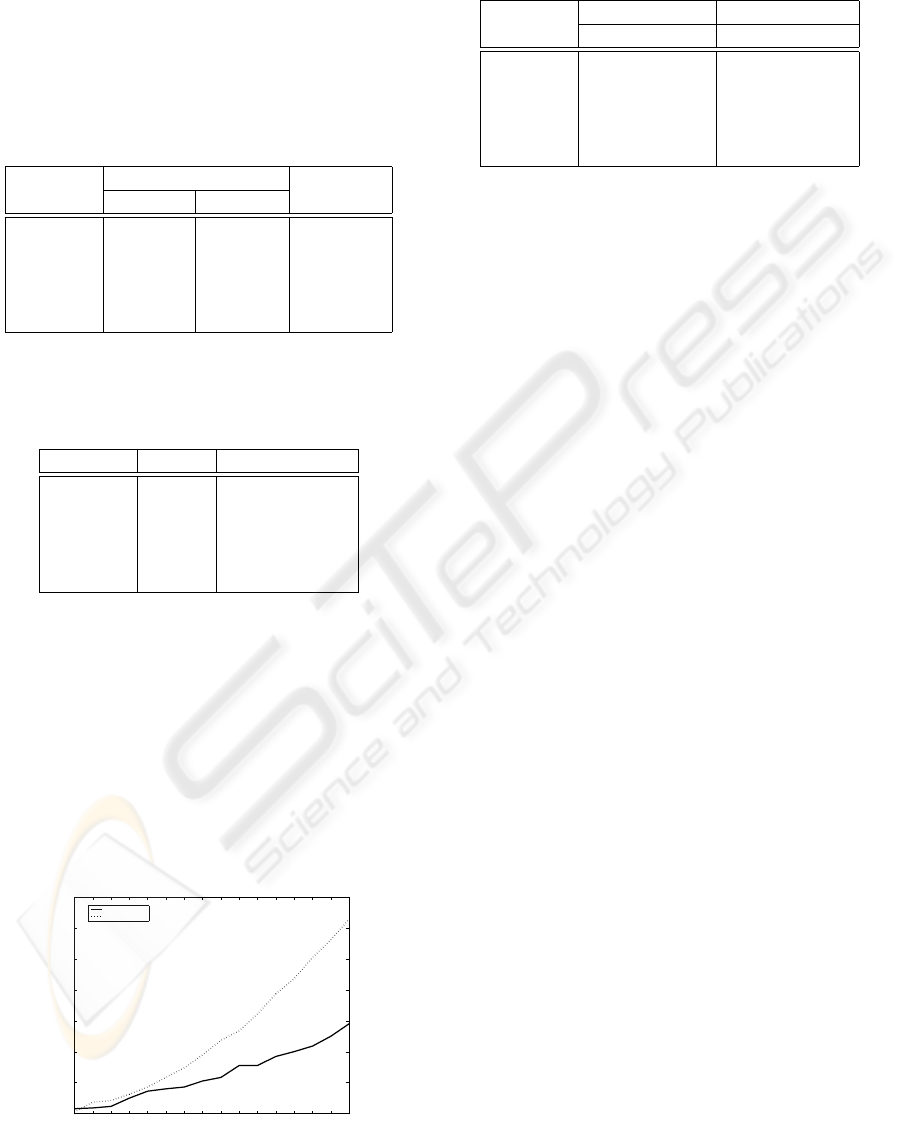
Figure 1: Comparison of training time curves with Gaussian

kernel neurons between ELM and Gram-Schmidt Orthonor-

malization for Airplane case.

Table 3: Comparison of Average Mean Training Time (sec-

onds).

Name ELM Gram-Schmidt

Training Time Training Time

Abalone 0.0717 0.0942

Airplane 0.0159 0.0234

Boston 0.0087 0.0187

Census 0.2853 0.4280

Elevators 0.0927 0.1449

The mean training time of ELM and Gram-

Schmidt orthonormalization neural networks with the

30th neuron are illustrated in Table 3. From Ta-

ble 3, we can know that neural networks without

orthonormalization transformation take less training

time than neural networks with orthonormalization

transformation. In the absence of orthonormaliza-

tion transformation, neural networks can have faster

training speed. Fig 1 records training time of Air-

plane case from 5th neuron to 80th neuron every 5

steps. Seen from Fig 1, with the growth of neu-

ron number, the difference in training time between

ELM and Gram-Schmidt orthonormalization neural

networks becomes greater, which further veriﬁes the

correctness of our conclusion.

5 CONCLUSION

An orthonormal kernel neural networks have been

proved to be a fast learning mechanism in (Kamin-

ski and Strumillo, 1997). However, in this paper, we

have rigorously proved and demonstrated that such

orthonormalization transformation is not necessary

for neural networks. Therefore neural networks with-

out orthonormalization transformation can run faster

than neural networks with orthonormalization trans-

formation while achieving the same generalization

performance. We have also extended in this paper

the applied scope of activation functions into addi-

tive neurons. Some benchmark regression problems

further verify our conclusion.

REFERENCES

Huang, G.-B., Zhu, Q.-Y., and Siew, C.-K. (2006). Extreme

learning machine: Theorey and applications. Neuro-

computing, 70:489–501.

Kaminski, W. and Strumillo, P. (1997). Kernel orthonormal-

ization in radial basis function neural networks. IEEE

Transactions On Neural Networks, 8(5):1177–1183.

FEEDFORWARD NEURAL NETWORKS WITHOUT ORTHONORMALIZATION

423