HIGHER-ORDER STATISTICS INTERPRETATION. APPLICATION
TO POWER-QUALITY CHARACTERIZATION
Juan Jos
´
e Gonz
´
alez de la Rosa,
´
Africa Luque
Univ. C
´
adiz. Electronics Area. Research Group PAI-TIC-168, EPSA. Av. Ram
´
on Puyol S/N. E-11202-Algeciras-C
´
adiz-Spain
Carlos G. Puntonet, J. M. G
´
orriz
Univ. Granada. Dept. ATC, ESII. Periodista Daniel Saucedo. E-18071-Granada-Spain
Antonio Moreno Mu
˜
noz
Univ. C
´
ordoba. Electronics Area. Research Group PAI-TIC-168
Campus Rabanales. A. Einstein C-2. E-14071-C
´
ordoba-Spain
Keywords:
Higher-Order statistics, Signal processing, Transient Characterization, Power-Quality.
Abstract:
In this paper we perform a practical review on higher-order statistics interpretation. Concretely we focuss
on an unbiased estimate of the 4th-order time-domain cumulants. Some synthetics involving classical noise
processes are characterized using this unbiased estimate, with the goal of checking its performance and to
provide the scientific community with another result, dealing with the interpretation of this signal processing
tool. A real-life practical example is presented in the field of electrical power quality event analysis. The work
also aims to present a set of general advice in order to save memory and gain speed in a real signal processing
frame, dealing with non-stationary processes.
1 INTRODUCTION
Gaussian processes are completely characterized
by the autocorrelation sequence and its associated
Fourier transform, the power spectrum. In the power
spectrum estimation, the information regarding the
phase of the frequency components of the signal is
not present. The information in the power spectrum is
essentially the same as in the autocorrelation (Nandi,
1999).
However, there are numerous situations where
we have to look beyond the autocorrelation in or-
der to get extra information regarding deviations from
the Gaussian behavior and nonlinear characteriza-
tion. These additional characteristics help us distin-
guish among apparently similar measurement data se-
quences; therefore getting the complete characteriza-
tion of the process.
Data sequences, and their associated power spec-
tra, which have been obtained by multiplying more
than two time-series are called higher-order statistics
(HOS). Their associated Fourier transforms are called
poly-spectra. They contain additional information re-
garding the phase of the frequency components of the
signals under study (Nikias and Petropulu, 1993).
The power spectrum (second-order spectrum) is
a particular case of higher-order spectra. The third-
order spectrum is called the bi-spectrum and the
fourth-order spectrum is called the try-spectrum.
They are defined to be the Fourier transforms or the
third and the fourth-order cumulant sequences, re-
spectively.
Poly-spectra are defined as the higher-order mo-
ment spectra and cumulant spectra can be defined for
both deterministic signals and random processes. Mo-
ment spectra can be very useful in the analysis of de-
terministic signals (transient and periodic), whereas
cumulant spectra are of great importance in the anal-
ysis of stochastic signals.
The motivation of the poly-spectral analysis yields
in three applications: (a) To suppress Gaussian noise
processes of unknown spectral characteristics; the bi-
spectrum also suppress noise with symmetrical prob-
ability distribution, (b) to reconstruct the magnitude
and phase response of systems, and (c) to detect and
characterize nonlinearities in time-series.
In this paper we show the application results deal-
ing with the characterization of random processes,
72
José González de la Rosa J., Luque Á., G. Puntonet C., M. Górriz J. and Moreno Muñoz A. (2007).
HIGHER-ORDER STATISTICS INTERPRETATION. APPLICATION TO POWER-QUALITY CHARACTERIZATION.
In Proceedings of the Second International Conference on Signal Processing and Multimedia Applications, pages 72-78
DOI: 10.5220/0002136100720078
Copyright
c
 SciTePress

following the indications in (Nandi, 1999) and in
(Nikias and Petropulu, 1993). A real example in-
volving power quality event analysis is then stud-
ied to show the difference in dealing with real time-
series instead of synthetics. Computational intelli-
gence based in neural classifiers are pointed as the
classification strategy, once the transients have been
characterized.
The paper is structured as follows. Section 2 in-
cludes the motivation of HOS and an amenable math-
ematical foundation. In Section 3 a time-domain
fourth-order cumulant analysis is applied to time se-
ries regarding realizations of noise processes. Section
4 presents the real-life analysis of electrical transients.
Finally, conclusions are shown in Section 5.
2 HOS IN TIME AND
FREQUENCY DOMAINS
2.1 A Preliminary Example
To motivate the use of HOS a first application is out-
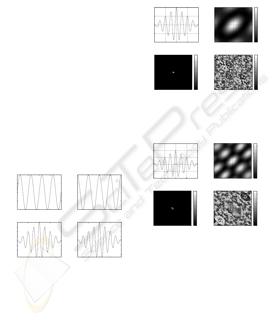
lined. We consider two cosine waves of the same fre-
quency with a phase shift of π/2 radians. The signals
and their autocorrelation plots are depicted in Fig. 1.
100 200 300 400
-1
-0.5
0
0.5
1
200 400 600 800
-150
-100
-50
0
50
100
150
200
100 200 300 400
-1
-0.5
0
0.5
1
200 400 600 800
-150
-100
-50
0
50
100
150
200
Figure 1: Two sinusoids with the same frequency, shifted
π/2 radians (Two upper graphs). They have the same
second-order statistics (the autocorrelation sequence).
Figs. 2 and 3 show the contour plots associated
to the third-order cumulant and the bi-spectrum of the
former cosine sequences. Qualitatively (but also in
almost every practical case) we only have to pay at-
tention at the coarser differences between graphs. The
main bump in the center of Fig. 2, which corresponds
to the situation of zero phase shift between the sinu-
soids, disappears in Fig. 3, giving rise to others, sec-
ondary bumps. Thanks to the bi-spectrum, these extra
bumps indicate by the way the presence of a phase
shift.
0 2 4 6 8
x 10
-3
-200
-100
0
100
200
Averaged Signal
Time (s )
Signal (V )
3
rd
Order Cumulant (V
3
)
Lag τ
0
(s )
Lag τ
1
(s )
-5 0 5
x 10
-4
-5
0
5
x 10
-4
-1
0
1
2
3
4
x 10
4
Bispectrum Magnitude (V
3
/Hz
2
)
Frequency f
0
(Hz )
Frequency f
1
(Hz )
-5 0 5
x 10
4
-5
0
5
x 10
4
1
2
3
4
x 10
7
Bispectrum Phase (deg )
Frequency f
0
(Hz )
Frequency f
1
(Hz )
-5 0 5
x 10
4
-5
0
5
x 10
4
-150
-100
-50
0
50
100
150
Figure 2: Third-order statistics of the autocorrelation func-
tion (top-left) corresponding to a sinusoid with no phase
shift. A main bump. in the center is observed in the cu-
mulant plot (top-right).
0 2 4 6 8
x 10
-3
-200
-100
0
100
200
300
Averaged Signal
Time (s )
Signal (V )
3
rd
Order Cumulant (V
3
)
Lag τ
0
(s )
Lag τ
1
(s )
-5 0 5
x 10
-4
-5
0
5
x 10
-4
-5000
0
5000
10000
15000
Bispectrum Magnitude (V
3
/Hz
2
)
Frequency f
0
(Hz )
Frequency f
1
(Hz )
-5 0 5
x 10
4
-5
0
5
x 10
4
2
4
6
8
10
12
14
x 10
6
Bispectrum Phase (deg )
Frequency f
0
(Hz )
Frequency f
1
(Hz )
-5 0 5
x 10
4
-5
0
5
x 10
4
-150
-100
-50
0
50
100
150
Figure 3: Third-order statistics of the autocorrelation func-
tion (top-left) corresponding to a sinusoid with a constant
90 phase shift. Several bumps. appear in the cumulant plot
(top-right).
Let’s revise some mathematical foundations.
2.2 Cumulants and Moments
High-order statistics, known as cumulants, are used to
infer new properties about the data of non-Gaussian
processes (Hinich, 1990; Mendel, 1991; Nikias and
Petropulu, 1993). Before cumulants, due to the lack
of analytical tools, such processes had to be treated as
if they were Gaussian. Cumulants and their associated
Fourier transforms, known as poly-spectra, reveal in-
formation about amplitude and phase, whereas sec-
HIGHER-ORDER STATISTICS INTERPRETATION. APPLICATION TO POWER-QUALITY CHARACTERIZATION
73

ond order statistics (power, variance, covariance and
spectra) are phase-blind (Mendel, 1991; Swami et al.,
2001; De la Rosa et al., 2005; De la Rosa and Ruz-
zante, 2007, ).
Before the definitions, it is convenient to remark
that cumulants of order higher than 2 are all zero in
signals with Gaussian probability density functions.
What is the same, cumulants are blind to any kind of
a Gaussian process. This is the reason why it is not
possible to separate these signals using the statistical
approach (Nikias and Petropulu, 1993).
The relationship among the cumulant of r stochas-
tic signals, {x
i
}
i∈[1,r]
, and their moments of order
p, p ≤ r, can be calculated by using the Leonov-
Shiryaev formula (Mendel, 1991; Nikias and Petrop-
ulu, 1993)
Cum(x
1
, ..., x
r
) =
(−1)
p−1
· (p − 1)! · E{
i∈s
1
x
i
}
· E{
i∈s
2
x
j
} · · · E{
i∈s
p
x
k
}
(1)
where the addition operator is extended over all
the partitions, like one of the form (s
1
, s
2
, · · · , s
p
),
p = 1, 2, · · · , r; and (1 ≤ i ≤ p ≤ r); s
i
is a set be-
longing to a partition of order p, of the set of integers
1,...,r.
For a zero mean variable, using (1), the second-
, third-, and fourth-order cumulants, are particular
cases and are given by:
Cum(x
1
, x
2
) = E{x
1
· x
2
} (2a)
Cum(x
1
, x
2
, x
3
) = E{x
1
· x
2
· x
3
} (2b)
Cum(x
1
, x
2
, x
3
,x
4
) = E{x
1
· x
2
· x
3
· x
4
}
− E{x
1
· x
2
}E{x
3
· x
4
}
− E{x
1
· x
3
}E{x
2
· x
4
}
− E{x
1
· x
4
}E{x
2
· x
3
}
(2c)
Let {x(t)} be an rth-order stationary random real-
valued process. The rth-order cumulant is defined as
the joint rth-order cumulant of the random variables
x(t), x(t+τ
1
),..., x(t+τ
r−1
),
C
r,x
(τ
1
, τ
2
, . . . , τ
r−1
)
= Cum[x(t), x(t + τ
1
), . . . , x(t + τ
r−1
)]
(3)
For stationary random processes the rth-order cu-
mulant is only a function of r-1 lags. If {x(t)} is non-
stationary then the rth-order cumulant includes time
dependency.
The second-, third- and fourth-order cumulants of
zero-mean x(t) can be expressed using (2) and (3), via
C
2,x
(τ) = E{x(t) · x(t + τ)} (4a)
C
3,x
(τ
1
, τ
2
) = E{x(t) · x(t + τ
1
) · x(t + τ
2
)} (4b)
C
4,x
(τ
1
, τ
2
, τ
3
)
= E{x(t) · x(t + τ
1
) · x(t + τ
2
) · x(t + τ
3
)}
− C
2,x
(τ
1
)C
2,x
(τ
2
− τ
3
)
− C
2,x
(τ
2
)C
2,x
(τ
3
− τ
1
)
− C
2,x
(τ
3
)C
2,x
(τ
1
− τ
2
)
(4c)
By putting τ
1
= τ
2
= τ
3
= 0 in Eq. (4), we obtain
γ
2,x
= E{x
2
(t)} = C
2,x
(0) (5a)
γ
3,x
= E{x
3
(t)} = C
3,x
(0, 0) (5b)
γ
4,x
= E{x
4
(t)} − 3(γ
2,x
)
2
= C
4,x
(0, 0, 0) (5c)
The expressions in Eq. (5) are measurements of
the variance, skewness and kurtosis of the distribu-
tion in terms of cumulants at zero lags (the central
cmulants).
Normalized kurtosis and skewness are defined as
γ
4,x
/(γ
2,x
)
2
and γ
3,x
/(γ
2,x
)
3/2
, respectively. We
will use and refer to normalized quantities because
they are shift and scale invariant. If x(t) is symmetri-
cally distributed, its skewness is necessarily zero (but
not vice versa); if x(t) is Gaussian distributed, its kur-
tosis is necessarily zero (but not vice versa).
2.3 Poly-spectra
We will assume in the following that the cumulant se-
quences satisfies the bounding condition:
τ
1
=+∞
X
τ
1
=−∞
· · ·
τ
r−1
=+∞
X
τ
r−1
=−∞
|C
r,x
(τ
1
, τ
2
, . . . , τ
r−1
)| < ∞
(6)
Under this assumption, the higher-order spectra
are usually defined in terms of the rth-order cumu-
lants as their (r-1)-dimensional Fourier transforms
S
r,x
(f
1
, f
2
, . . . , f
r−1
)
=
τ
1
=+∞
X
τ
1
=−∞
· · ·
τ
r−1
=+∞
X
τ
r−1
=−∞
C
r,x
(τ
1
, τ
2
, . . . , τ
r−1
)
· exp[−j2π(f
1
τ
1
+ f
2
τ
2
+ · · · + f
r−1
τ
r−1
)]
(7)
The special poly-spectra derived from (7) are
power spectrum (r=2), bi-spectrum (r=3) and try-
spectrum (r=4). Only power spectrum is real, the oth-
ers are complex magnitudes.
SIGMAP 2007 - International Conference on Signal Processing and Multimedia Applications
74

Poly-spectra are multidimensional functions
which comprise a lot of information. As a con-
sequence, their computation may be impractical
in some cases. To extract useful information
one-dimensional slices of cumulant sequences and
spectra, and bi-frequency planes are employed in
non-Gaussian stationary processes (Jakubowski et al.,
2002), (De la Rosa et al., 2004, ).
3 ESTIMATES AND
CHARACTERIZATION OF
STATISTICAL PROCESSES
In this section we show the computation results ob-
tained from the application of an estimator. In prac-
tice, the computation of the cumulants and the poly-
spectra is based in estimates. In order to asses the
performance of the selected estimator we test it con-
sidering a 2048-point sample register for each noise
process, as it was catalogued in (Nikias and Petrop-
ulu, 1993). These four noise processes are indistin-
guishable from the second-order perspective, as it is
shown in 4.
−20 −15 −10 −5 0 5 10 15 20
−0.5
0
0.5
1
Gaussian
Second−order cumulants: Autocorrelation sequences
−20 −15 −10 −5 0 5 10 15 20
−0.5
0
0.5
1
Uniform
−20 −15 −10 −5 0 5 10 15 20
−0.5
0
0.5
1
Exponential
−20 −15 −10 −5 0 5 10 15 20
−0.5
0
0.5
1
lag
Laplacian
Figure 4: The four second-order cumulants corresponding
to 4 sample registers, each of which is a realization of a dif-
ferent noise process. They exhibit the same autocorrelation
sequence.
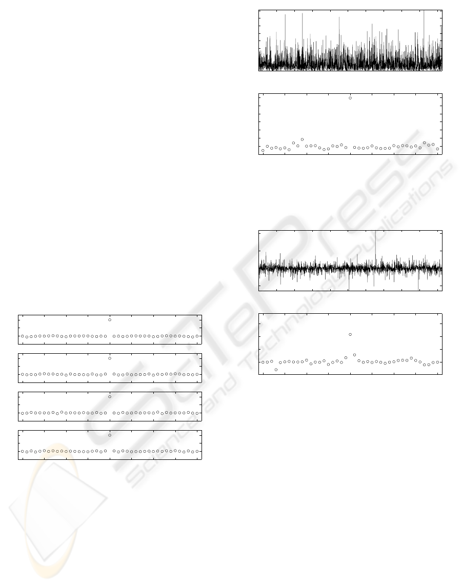
If we look into the fourth-order sequences, sub-
stantial differences are observed, specially those cor-
responding to zero time lags. This can be seen in Figs.
form 5 to 8.
200 400 600 800 1000 1200 1400 1600 1800 2000
0
1
2
3
4
5
6
7
Sample number
Exponentially distributed random process
−20 −15 −10 −5 0 5 10 15 20
−1
0
1
2
3
4
5
6
lag, τ
1
c
4,x
(τ
1
,0,0)
c
4,x
(τ
1
,0,0); τ
2
=τ
3
=0
Figure 5: A 2048-point realization of an exponentially dis-
tributed noise process. Maximum value (at zero lag) =
5.9326585626518 (theoretical=6).
200 400 600 800 1000 1200 1400 1600 1800 2000
−5
0
5
10
Sample number
Laplacian distributed random process
−20 −15 −10 −5 0 5 10 15 20
−5
0
5
10
15
τ
1
c
4,x
(τ
1
,0,0)
c
4,x
(τ
1
,0,0); τ
2
=τ
3
=0
Figure 6: A 2048-point realization of an Laplacian dis-
tributed noise process. Maximum value (at zero lag) =
10.7788 (theoretical=12).
4 FEATURE EXTRACTION IN
ELECTRICAL POWER EVENT
ANALYSIS
The aim of the experiment is to differentiate between
two classes of transients (PQ events), named long-
duration and short-duration. The experiment com-
prises two stages. The feature extraction (classifica-
tion) stage is based on the computation of the cumu-
lants (De la Rosa et al., 2007, ). Each vector’s coordi-
nate corresponds to the local maximum and minimum
of the 4th-order central cumulant. This is the feature-
extraction stage. And the classification stage is based
on the application of the competitive layer to the fea-
ture vectors, in order to obtain two clusters in the fea-
ture plane. We use a two-neuron competitive layer,
HIGHER-ORDER STATISTICS INTERPRETATION. APPLICATION TO POWER-QUALITY CHARACTERIZATION
75

200 400 600 800 1000 1200 1400 1600 1800 2000
−2
−1
0
1
2
3
Sample number
Gaussian distributed random process
−20 −15 −10 −5 0 5 10 15 20
−0.1
−0.05
0
0.05
0.1
0.15
τ
1
c
4,x
(τ
1
,0,0)
c
4,x
(τ
1
,0,0); τ
2
=τ
3
=0
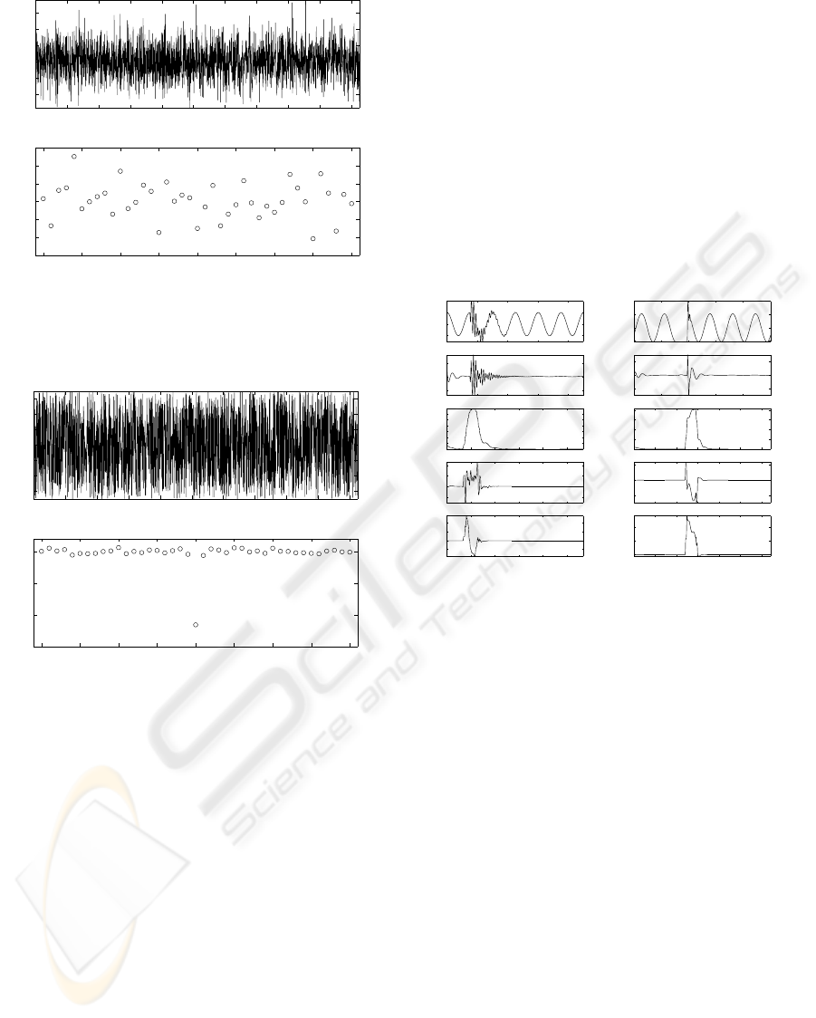
Figure 7: A 2048-point realization of an Gaussian dis-
tributed noise process. Extreme value not defined; al the
values surrounds zero.
200 400 600 800 1000 1200 1400 1600 1800 2000
−1.5
−1
−0.5
0
0.5
1
1.5
Sample number
Uniformly distributed random process
−20 −15 −10 −5 0 5 10 15 20
−1.5
−1
−0.5
0
lag, τ
1
c
4,x
(τ
1
,0,0)
c
4,x
(τ
1
,0,0); τ
2
=τ
3
=0
Figure 8: A 2048-point realization of a uniformly dis-
tributed noise process. Extreme value (for zero lag) = -
1.15845526517794 (theoretical=-1).
which receives two-dimensional input feature vectors
in this training stage.
We analyze a number of 16 1000-point (roughly)
real-life registers during the feature extraction stage.
Before the computation of the cumulants, two pre-
processing actions have been performed over the sam-
ple signals. First, they have been normalized because
they exhibit very different-in-magnitude voltage lev-
els. Secondly, a high-pass digital filter (5th-order But-
terworth model with a characteristic frequency of 150
Hz) eliminates the low frequency components which
are not the targets of the experiment. This by the way
increases the non-Gaussian characteristics of the sig-
nals, which in fact are reflected in the higher-order
cumulants.
After filtering, a 50-point sliding battery of cen-
tral cumulants (2nd, 3rd and 4th order) are calculated.
The window’s width (50 points) has been selected nei-
ther to be so long to cover the whole signal nor to be
very short. The algorithm calculates the 3 central cu-
mulants over 500 points, and then it jumps to the fol-
lowing starting point; as a consequence we have 98
per cent overlapping sliding windows (49/50=0.98).
Thus, each computation over a window (called a seg-
ment) outputs 3 cumulants.
Fig. 9 shows an example of signal processing
analysis of two sample registers corresponding to
a long-duration and a short-duration events, respec-
tively.
0.02 0.04 0.06 0.08
−0.5
0
0.5
1
Analysis of a long−duration transient
0.02 0.04 0.06 0.08
−0.5
0
0.5
Time(s)
100 200 300 400 500
0.02
0.04
0.06
0.08
0.1
0.12
2
nd
−order sliding cumulant
100 200 300 400 500
−5
0
5
10
x 10
−3
3
rd
−order sliding cumulant
100 200 300 400 500
−5
0
5
10
x 10
−3
Number of segment
4
th
−order sliding cumulant
0.02 0.04 0.06 0.08 0.1
−0.5
0
0.5
1
Analysis of a short−duration transient
0.02 0.04 0.06 0.08 0.1
−0.5
0
0.5
Time(s)
100 200 300 400 500 600
0.02
0.04
0.06
0.08
2
nd
−order cumulant
100 200 300 400 500 600
−0.01
0
0.01
3
rd
−order cumulant
100 200 300 400 500 600
0
5
10
x 10
−3
Number of segment
4
th
−order cumulant
Figure 9: Long-duration vs. short-duration transient anal-
ysis. From top to bottom: the original data record, the fil-
tered sequence, 2nd-3rd-4th-order cumulants sliding win-
dows, respectively.
The 2nd-order cumulant sequence corresponds to
the variance, which clearly indicates the presence of
an event, due to the excess of power. Both types
of transients exhibit an increasing variance in the
neighborhood of the PQ event, that presents the same
shape, with only one maximum. The magnitude of
this maximum is by the way the only available feature
which can be used to distinguish different events from
the second-order point of view. This may suggest the
use of additional features in order to distinguish dif-
ferent types of events.
For this reason the higher-order central cumu-
lants are chosen. An unbiased estimator of the cu-
mulants has been selected. Third-order diagrams
don’t show quite different clusters if we consider a
bi-dimensional space (2 coordinates for each feature
vector) because maxima and minima are similar. It is
possible to differentiate PQ events from the 3rd-order
perspective if we consider more features in the input
vector, like the number of extremes (maxima and min-
ima), and the order in which the maxima and the min-
SIGMAP 2007 - International Conference on Signal Processing and Multimedia Applications
76

ima appear as time increases. In this paper we have
focussed the experience on a bi-dimensional represen-
tation (2-dimensional feature vectors) because we ob-
tain very intelligible 2-D graphs.
Fourth-order sliding cumulants exhibit clear dif-
ferences, not only for the shape of the computation
graph (the bottom graphs in Fig. 9, but also for the
different location of minima, which suggest a cluster-
ing zone for the points.
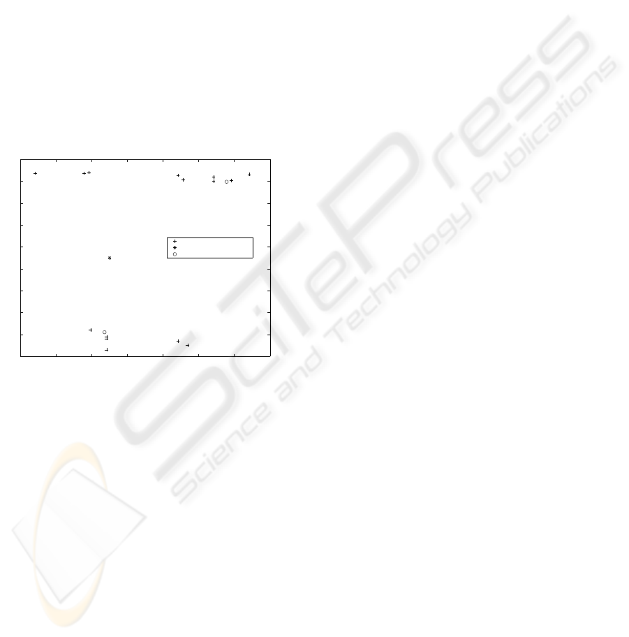
Fig. 10 presents the results of the training stage,
using the Kohonen rule. The horizontal (vertical) axis
corresponds to the maxima (minima) value. Each
cross in the diagram corresponds to an input vector
and the circles indicate the final location of the weight
vector (after learning) for the two neurons of the com-
petitive layer. Both weight vectors point to the aster-
isk, which is the initializing point (the midpoint of the
input intervals).
0.03 0.04 0.05 0.06 0.07 0.08 0.09 0.1
−9
−8
−7
−6
−5
−4
−3
−2
−1
0
x 10
−3
Cluster classification. 4th−order cumulant
cumulant maxima
cumulant minima
:measured vector
:initial neuron weight vector
:final neuron weight vector
Figure 10: Competitive layer training results over 20
epochs. Upper cluster: Short-duration PQ-events. Down
cluster: Long-duration event.
The separation between classes (inter-class dis-
tance) is well defined. Both types of PQ events are
horizontally clustered. The correct configuration of
the clusters is corroborated during the simulation of
the neural network, in which we have obtained an ap-
proximate classification accuracy of 97 percent. Dur-
ing the simulation new signals (randomly selected
from our data base) were processed using the method
described.
The accuracy of the classification method in-
creases with the number of data. To evaluate the con-
fidence of the statistics a significance test have been
conducted. This informs if the number of experiments
is statistically significant according to the fitness test
(
¨
Omer Nezih Gerek and Ece, 2006). As a result of
the test, the number of measurements is significatively
correct.
5 CONCLUSION
In this work we have reviewed computation of higher-
order statistics. Concretely we have focussed on a
4-order estimates. We have also proposed a method
to detect and classify two electrical power transients,
named short and long-duration. The method com-
prises two stages. The first includes pre-processing
(normalizing and filtering) and outputs the 2-D fea-
ture vectors, each of which coordinate corresponds to
the maximum and minimum of the central cumulants.
The second stage uses a neural network to classify the
signals into two clusters. This stage is different-in-
nature from the one used in (
¨
Omer Nezih Gerek and
Ece, 2006) consisting of quadratic classifiers. The
configuration of the clusters is assessed during the
simulation of the neural network, in which we have
obtained an acceptable classification accuracy.
ACKNOWLEDGEMENTS
The authors would like to thank the Spanish Min-
istry of Education and Science for funding the project
DPI2003-00878 which involves noise processes mod-
eling, and the PETRI project PTR95-0824-OP in-
volving higher-order statistics. Also thanks to the
Andalusian Government for the trust put in the re-
search group PAI-TIC-168, and for supporting the ex-
cellence project PAI2005-TIC00155, which involves
higher-order statistics.
REFERENCES
Hinich, M. J. (1990). Detecting a transient signal
by biespectral analysis. IEEE Trans. Acoustics,
38(9):1277–1283.
Jakubowski, J., Kwiatos, K., Chwaleba, A., and Osowski,
S. (2002). Higher order statistics and neural network
for tremor recognition. IEEE Trans. on Biomedical
Engineering, 49(2):152–159.
Mendel, J. M. (1991). Tutorial on higher-order statistics
(spectra) in signal processing and system theory: The-
oretical results and some applications. Proceedings of
the IEEE, 79(3):278–305.
Nandi, A. K. (1999). Blind Estimation using Higher-Order
Statistics, volume 1. Kluwer Academic Publichers,
Boston, 1 edition.
Nikias, C. L. and Petropulu, A. P. (1993). Higher-Order
Spectra Analysis. A Non-Linear Signal Processing
Framework. Englewood Cliffs, NJ, Prentice-Hall.
¨
Omer Nezih Gerek and Ece, D. G. (2006). Power-
quality event analysis using higher order cumulants
HIGHER-ORDER STATISTICS INTERPRETATION. APPLICATION TO POWER-QUALITY CHARACTERIZATION
77

and quadratic classifiers. IEEE Transactions on Power
Delivery, 21(2):883–889.
Swami, A., Mendel, J. M., and Nikias, C. L. (2001).
Higher-Order Spectral Analysis Toolbox User’s
Guide.
De la Rosa, J. J. G., Lloret, I., Puntonet, C. G., and G
´
orriz,
J. M. (2004). Higher-order statistics to detect and
characterise termite emissions. Electronics Letters,
40(20):1316–1317. Ultrasonics.
De la Rosa, J. J. G., Moreno, A., Lloret, I., Puntonet,
C. G., and G
´
orriz, J. M. (2007). Power tran-
sients characterization and classification using higuer-
order cumulants and competitive layers. Lecture
Notes in Computer Science (LNCS), 4431:782–789.
International Conference on Adaptative and Natu-
ral Computung Algorithms, ICANNGA 2007 War-
saw, Poland, April 11-14, 2007, Proceedings, Part I;
http://icannga07.ee.pw.edu.pl/.
De la Rosa, J. J. G., Puntonet, C. G., and Lloret, I. (2005).
An application of the independent component analy-
sis to monitor acoustic emission signals generated by
termite activity in wood. Measurement (Ed. Elsevier),
37(1):63–76. Available online 12 October 2004.
De la Rosa, J. J. G. and Ruzzante, R. P. J. (2007). Third-
order spectral characterization of acoustic emission
signals in ring-type samples from steel pipes for the
oil industry. Mechanical systems and Signal Process-
ing (Ed. Elsevier), 21(Issue 4):1917–1926. Available
online 10 October 2006.
SIGMAP 2007 - International Conference on Signal Processing and Multimedia Applications
78