VISUALIZING COLLAPSIBLE 3D DATA IN A HYBRID GIS
Stephen Brooks
Faculty of Computer Science, Dalhousie University, 6050 University Avenue, Halifax, Canada
Jacqueline Whalley
School of Computer and Information Sciences, Auckland University of Technology, Auckland, New Zealand
Keywords: 2D and 3D visualization, geographical information systems, hybrid display, interactive.
Abstract: In this paper we present a comprehensive set of advancements to our unique hybrid Geographical
Information System (GIS). Although many existing commercial 3D GIS systems offer 2D views they are
typically isolated from the 3D view in that they are presented in a separate window. Our system is a novel
hybrid 2D/3D approach that seamlessly integrates 2D and 3D views of the same data. In our interface,
multiple layers of information are continuously transformed between the 2D and 3D modes under the
control of the user, directly over a base-terrain. In this way, our prototype GIS allows the user to view the
2D data in direct relation to the 3D view within the same window. In this work we progress the concept of a
hybrid GIS by presenting a set of expanded capabilities within our distinctive system. These additional
facilities include: landmark layers, 3D point layers, and chart layers, the grouping of multiple hybrid layers,
layer painting, the merging of layer controls and consistent zooming functionality.
1 INTRODUCTION
In the past, most geographical information systems
(GIS) were limited to providing visualizations of
data in 2D. Currently, GIS research and
development still lies largely in this traditional map-
based approach. But we relate to our world in three
or more dimensions, which suggests that some types
of data may be more readily visualized and analyzed
in 3D. However, direct 3D analogues to 2D GIS are
not ideal solutions because they suffer from several
shortcomings and gaining insight from 3D spatial
datasets can be particularly challenging.
One issue is that a high data density can make it
difficult to view all the data at once due to the self-
occlusion of the data. The issue can be particularly
acute when attempting to display and interpret
multivariate data in a meaningful way. Moreover,
there can arise difficulties in viewing information in
3D GIS when the terrain is hilly due to elevated
regions in the terrain occluding data. How best to
simultaneously visualize different types of data in
3D is another key issue.
Studies have shown that 2D views are often used
to establish precise relationships, while 3D views
help in the acquisition of qualitative understanding
(Springmeyer et al., 1992). Both dimensionalities of
view therefore have distinct advantages and it would
be ideal if the benefits of both 2D and 3D could be
incorporated into the same system.
Our hybrid system seamlessly integrates 2D and
3D views of the same data and allows the user to
view the 2D data in direct relation to the 3D view
within the same window. Our system visualizes
layers in a combined overlay representation where
multiple heterogeneous layers of information are
continuously transformed between 2D and 3D over
the base-terrain (see Figure 1). It is intended that this
system allows the exploration and understanding of
structures, patterns and processes reflected in both
2D and 3D data.
In this paper, we present a set of expanded
capabilities for our unique GIS which include:
hybrid landmark and chart layers, 3D point layers,
the aggregate grouping of multiple hybrid layers,
layer painting, unified controls for layer groups and
consistent zooming functionality.
171
Brooks S. and Whalley J. (2007).
VISUALIZING COLLAPSIBLE 3D DATA IN A HYBRID GIS.
In Proceedings of the Second International Conference on Computer Graphics Theory and Applications - AS/IE, pages 171-178
DOI: 10.5220/0002075901710178
Copyright
c
 SciTePress

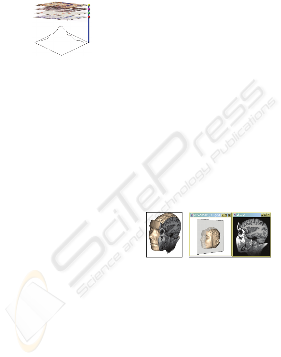
Figure 1: Multiple 2D/3D layers in our hybrid display over
a 3D base terrain. The vertical translation of each layer is
set with its associated control ball.
2 RELATED WORK
In recent years, GIS has gradually been moving into
the third dimension. 3D GIS have received
considerable attention and the literature surrounding
the area is slowly growing. In 2002, Zlatanova et al.
produced a survey of mainstream GIS software.
They reviewed a number of systems including:
ArcGIS (ESRI, 2006) and PAMAP GIS
Topographer (PAMAP, 2006). They concluded that
some initial steps forward have been made in terms
of the visualization of 3D spatial data, however, 3D
GIS still lack basic 2D GIS functions.
Further examples of existing 3D GIS include
systems such as Terrafly (Rishe et al., 1999),
GeoVR (Huang and Lin, 2002), TerraVisionII
(Reddy et al., 1999), GeoZui3D (Ware et al., 2001)
and VGIS (Köller et al., 1995). One noteworthy
system, called GeoTime (Kapler and Wright, 2005)
proposes an interesting solution to the problem of
integrating timeline events into interactive GIS.
Recently, Stota and Zlatnaova (Stota and Zlatanova,
2003) revisited the current status of 3D GIS and
postulated that 3D GIS is merely at a point where
2D GIS was several years ago.
Several of the aforementioned GIS have the
capability of creating 3D perspective images using
elevation data. Often this is simply used for
illustration or fly-bys, with limited analysis of this
perspective imagery. These perspective renderings
are generally accepted as showing the relationships
of the GIS data to the natural terrain, but have
limited the efficacy of the perspective images to
'show and tell' type applications (Stota and
Zlatanova, 2003). Moreover, these representations
only permits the user to view map layers as a single
entity rather than being able to visualize the layers in
a combined overlay representation.
Further research is required to explore the
possibilities and constraints of 3D GIS in order to
move beyond simple flybys and map-making.
Indeed this is the definitive aim of the research
presented in this paper. But, gaining insight from 3D
spatial datasets can be particularly challenging
because a high data density can make it difficult to
view all data at once since the data can self-occlude.
There are also difficulties viewing information in 3D
GIS when the terrain is hilly due to elevated regions
in the terrain occluding data further back.
Attempts to overcome these issues in 3D GIS
usually involve displaying the terrain from several
different viewpoints in separate windows (Verbee et
al., 1999). However, separate views introduce new
problems since the integration and interpretation of
the multiple views must occur in the mind of the
user. It therefore places extra demands on the GIS
professional or casual GIS user. Another issue is
that the more views are displayed, the smaller each
view must be rendered for a fixed screen size.
We propose that by providing 2D-to-3D
transitional layers we can overcome both the self-
occlusion and terrain-occlusion issues. Our layering
system also offers a convenient means of handling
multiple heterogeneous sets of aspatial data under
user control. Additionally, the system allows the
user to temporarily set aside data that is not currently
relevant. Our work builds upon 3D GIS and is also
somewhat related to a small number of systems that
have been proposed in the area of scientific
visualization.
Figure 2: Medical clip-planes (left) and orientation icons
(right).
Medical displays sometimes incorporate aspects
of 2D and 3D in some fashion, and so, we now
review these systems. Medical scans, such as
Magnetic Resonance Imaging and Computed
Tomography, allow users to interact with a data. 2D
slices can be combined with a 3D overview using
one of two main approaches: clip planes and
orientation icons (Tory and Swindells, 2003). Clip
planes show slice details in their exact relative
position to the 3D context (figure 2, left). Whereas,
in orientation icon systems (figure 2, right), the 3D
overview and 2D details are in separate windows.
But, as will be seen, these systems are quite different
from ours.
GRAPP 2007 - International Conference on Computer Graphics Theory and Applications
172

For GIS, little has been done with respect to
hybrid displays. This is despite the fact that this type
of display allows the dual strengths of 2D and 3D
visualization to be exploited (Tory and Swindells,
2003). What follows is an in-depth discussion of
our hybrid GIS display and its implementation. In
section 3 we briefly review the key features of our
GIS. We follow this in section 4 with a discussion
of the set of novel advancements to the GIS that we
have recently designed and developed. In closing
we offer a set of future directions and conclude with
a summary of contributions.
3 THE HYBRID GIS
It is necessary to begin with a review of our hybrid
GIS for the present work to be understood. Our
prototype offered a preliminary set of features, as
was reported in an initial paper (Anonymous, 2005).
3.1 Rendering of the Base Terrain
The base terrain consists of a Digital Elevation
Model (DEM) dataset. Two approaches are available
for constructing a 3D model from DEM data. The
first approach is to use Triangulated Irregular
Network and the second is simply a regular grid.
Our terrain can incorporate satellite imagery and in
the absence of good satellite images, procedural
textures are generated based on DEM data. Much of
the data we used to develop our system was acquired
from the San Francisco Regional Database and the
U.S. Geological Survey repository. Our terrain data
is extracted from the DEM format and vector data
from the DLG format.
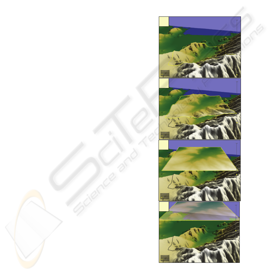
3.2 The Hybrid 2D/3D Layer System
What makes our GIS unique is the multiple layers of
information that can be continuously raised or
lowered by the user directly over the base-terrain.
During elevation, the transitional layers maintain
their original geographical (latitude/longitude)
position relative to the base terrain. When translated
skywards, the height values are gradually flattened
into a completely flat 2D map layer (figure 3a-c).
Each layer’s translation is set with an associated
user-positioned control ball. These control balls are
shown to the right in figure 3 and diagrammatically
in figure 1. The color of the control ball is unique for
each layer. In addition the layer is trimmed along its
edge with the same color as its associated control
ball. For example, in figure 3 the layer and control
ball are color coded yellow. This application of
consistent color coding finds support in user
interface design principles (Hix and Hartson, 1993).
When a layer is high above the terrain, it flattens
out to a true 2D map. This allows the user to analyze
information in 2D and also provides a way of
viewing information that may have been hidden by
near elevations in the 3D view. It also allows the
user to move information out of view when he or she
is not interested in the content of a particular layer.
This is achieved by simply raising the layer to the
top of the screen (Figure 3d).
Figure 3: The layer is shown gradually rising from image
a to image d. As the layer rises it morphs into a flat plane.
Image c shows the layer completely flat. Above the flat
level, the layer becomes increasingly transparent as shown
in image d.
c
a
b
d
VISUALIZING COLLAPSIBLE 3D DATA IN A HYBRID GIS
173

At a certain height the layer becomes flat, and
above this height the layer becomes increasingly
transparent, until all that is visible is its colored
outline which trims the layer’s edge. The trim is not
affected by the change in transparency.
It is important that the user is able to mentally
map a flattened 2D layer to the 3D terrain that it is
residing over. To aid this, a ground level shadow of
the layer system is provided which indicates the
correlation between the data in the 2D/3D layers and
the 3D base terrain.
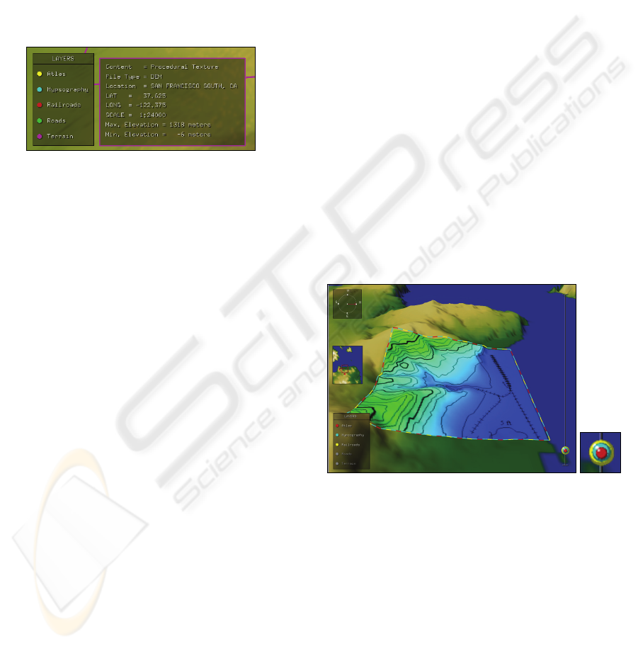
Figure 4: Text based meta-data pop-up legend for a layer.
In our initial prototype system we presented a
number of thematic layers in addition to the terrain
layer. These included a number of vector line data
layers (such as road and hypsography layers) and
color coded texture layers (such as an atlas layer).
Each of these layers required that its own meta-data
be available in an auxiliary pop-up legend (figure 4).
In section 4 we expand the range of possible hybrid
layers; in particular we will allow a variety of 3D
objects to be embedded in layers.
4 NEW HYBRID GIS FACILITIES
This section expands the capabilities of our
distinctive hybrid GIS. We first discuss the
aggregate grouping of layers, unified control
mechanism for the grouped constituents, and direct
layer painting. We then introduce several new types
of 3D layer content including: landmark layers, chart
layers and 3D point layers. The last subsection
discusses a consistent zooming capability.
4.1 Layer Grouping
Our layering system offers a convenient means of
handling multiple heterogeneous sets of aspatial data
by separating the data content into hybrid layers,
with each layer’s height controllable via its
associated control ball. We now add the ability to
group two or more layers into a single entity. The
user can form a new layer group simply by raising
(or lowering) layer A’s control ball onto the control
ball of layer B. The only required difference in the
interaction is that the user must drag the control ball
of layer A with the right mouse button (rather than
the usual left button). Layers can also be added to an
existing group by dragging additional control balls
to the same height (again with the right mouse
button pressed). An example of three grouped layers
is shown in figure 5, left. The layers are: atlas,
railroads and hypsography.
When multiple layers are grouped it is important
to provide a visual indication of the grouping and of
the individual member layers. We achieve this in
two complementary ways. Firstly, the edge trim that
surrounds each layer is adapted to the grouped state.
Each of the representative colors for each of the
layers is incorporated into the new edge trim in an
alternating dash pattern. Secondly, we alter the
control balls into onion-like configuration. We use
the term onioning to describe how the control balls
of grouped layers collected and visualized. We
display the combined control balls as if they are each
a layer of an onion that has been sliced in half. This
offers a further visual cue to the user and is also a
practical means of control. An example of the
alternating color trim and the combined control balls
for three layers is shown in figure 5.
Figure 5: Left: Multiple thematic layers grouped into a
single unit. Right: close-up of multiple control balls in an
united state. Also note the layer edge trim pattern which
has a matching color set.
Once a group is formed, the user can drag all
united control balls at once with the left mouse
button to raise and lower the combined layers as a
single entity. The flattening of layers into 2D and the
transparency of layers at a top height proceed as
normal. To separate a layer from a group, the user
simply drags the grouped control ball (again with the
right mouse button). We refer to this reverse
process as de-onioning. The layer that was added
last to the group is removed first. This is in keeping
GRAPP 2007 - International Conference on Computer Graphics Theory and Applications
174

with the onion metaphor, in that we are peeling outer
layers off the united group.
We also need to clarify exactly how layers are
shown with respect to other layers in the same
group. For this we need to consider the interaction
of three types of layer: 2D raster (image or array
data based), 2D vector (line-based) and 3D layers.
A selection of 3D layers is discussed in sections 4.2-
4.4. We first briefly list a number of cases that do
not pose difficulties:
1. Multiple vector layers, since vector lines do
not occlude.
2. Vector layers with a single raster layer, since
vector layers can be placed slightly above
the single raster layer, without occlusion.
3. One or more 3D layers with vector layers
and a single raster layer.
However, the case that does pose difficulties is
using multiple raster layers in a single group, as they
completely occlude each other. To overcome this
issue, we introduce the notion of direct layer
painting which allows the user to reveal the data
contained in one raster layer at the expense of all
other raster layers in the same group. This effect is
localized to wherever the user ‘paints’.
Let us consider an example layer group that
contains 3 raster layers added in this order: A, B and
C. Initially, the raster layer that is completely
visible is the first layer, A, that was added to the
group. Layers B and C are not initially visible. This
default arrangement may not be sufficient as the user
may wish to see certain portions of all three layers,
A, B, and C, at the same time.
To tailor visibility within the group, the user
performs layer painting. The user first clicks on the
name of the layer (within the layer legend) that he or
she wishes to reveal portions of. We will assume
this is layer B. The user then paints with the mouse
directly onto the rendered area of the layer group.
The areas that the user paints over will then only
show raster information contained within layer B,
thereby hiding data from layers A and C. The user
can therefore adjust the visibility of all layers in a
given group in this fashion, by constructing disjoint
sets of visible data from layers A, B and C.
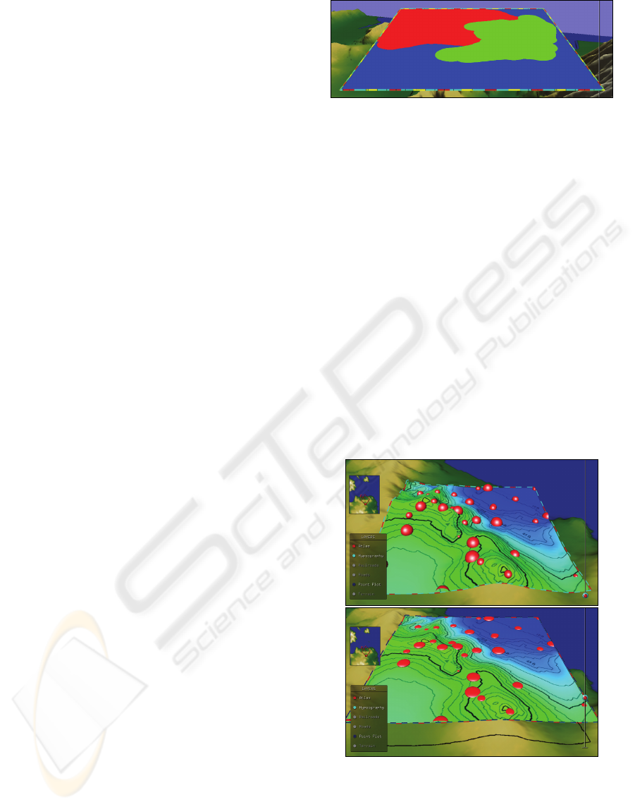
Figure 6 shows an example of this where 3
disjoint regions are shown painted for the 3 separate
raster layers within the same group. Note that the
regions have been colour coded in this figure
illustrate the concept. Normally, the corresponding
raster data from the 3 layers would be shown.
Figure 6: Colour coded disjoint regions shown painted for
3 separate raster layers in a layer group.
4.2 Point Layers
Point layers are standard in traditional 2D GIS; in
our system each point of data can be represented by
a 3D sphere (figure 7). The size of the sphere can
represent one aspatial aspect of the data points. For
example, if each data point represents the population
of a town, the location of the sphere could represent
the spatial data for the town. The size of the sphere
can then represent an aspatial data value for that
town, such as the population density value.
Each sphere is embedded in a layer and as the
layer flattens, the spheres also flatten to form a 2D
view. The spheres also become transparent with the
layer if the layer is raised sufficiently high. Also, it
is possible to form multiple point-layers for different
data content. Each point-layer is assigned its own
color and meta-data legend entry.
Figure 7: A partially transitioned point layer using sphere
and disk symbols.
VISUALIZING COLLAPSIBLE 3D DATA IN A HYBRID GIS
175

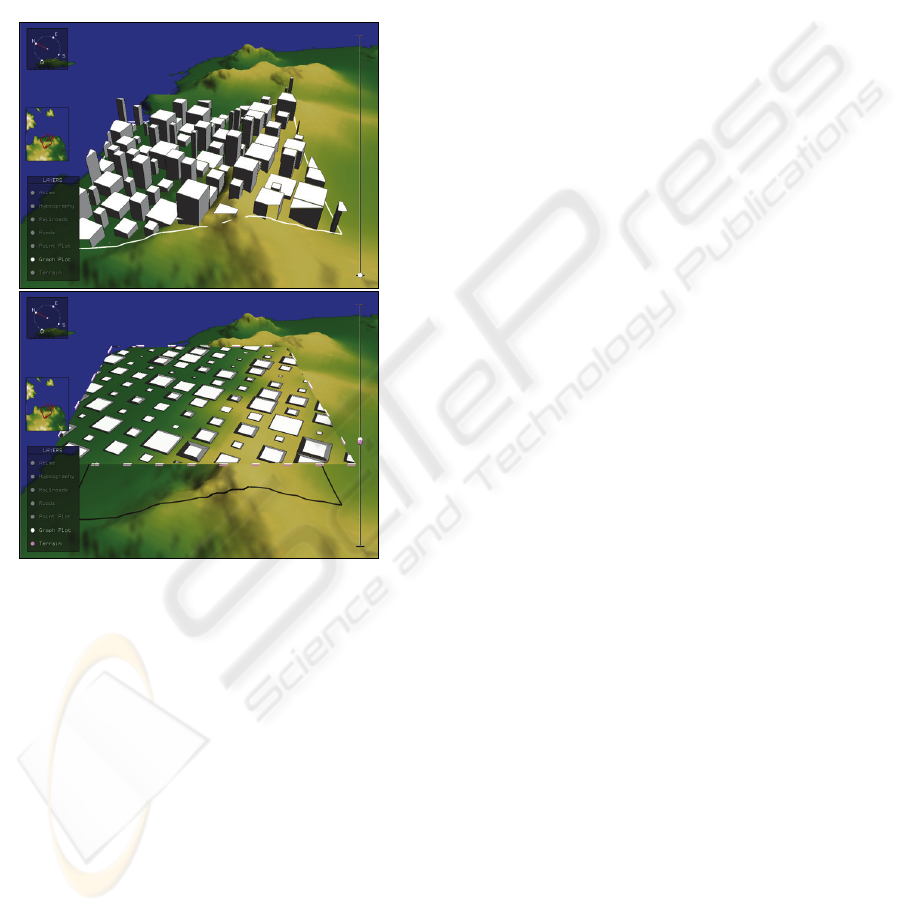
4.3 Landmark Layers
We have also integrated higher levels of detail into
our GIS. Our system now includes representations of
major landmarks such as buildings in a cityscape
(figure 8, top). As a cityscape is raised using the
associated control ball, the buildings flatten
gradually becoming 2D. And as with other map
layer types, when the layer is at the top of the
elevation bar the landmarks become translucent.
Figure 8: A landmark layer a ground-level (top) and at the
flattening level (bottom).
As the landmark layer flattens, 3D the buildings
become 2D polygons on a 2D plane. During this
flattening process the spatial information provided
by the 3D view with respect to the relative building
heights is lost. As a consequence, we have integrated
visuals cues for the height of building when flat.
For this, we add a scaled edge trim for each
building, indicative of the building’s height when
visualized in 2D (figure 8, bottom). This scaled edge
trim is implemented by scaling the top of the 3D
building inwardly, proportional to the height of the
building. In other words, the taller the building, the
more of an 'edge' there is around the building when
flat. This gives cue as to the building height even
though the building is 2D.
The inward scaling factor, f, for the tops of the
buildings, is calculated as:
sppspf )1(),( −
+
=
(1)
where:
))/1,0max(,1min( cHhp +
−
=
(2)
)/(1 Bbs
−
=
(3)
h is current layer height,
H is the height at which layers become flat,
b is the current building's height,
B is the height of the tallest building, and
c is the minimum scale factor (default = 0.5).
Equation 3 computes a scaling factor, s, which
scales the tops of taller buildings more than shorter
buildings. Equation 2, places limits on this scaling
so that the tops of the tallest buildings do not scale to
a zero size. Equation 2 also takes into account the
current layer height with respect to the maximum
allowable layer height. In practice, this will mean
that the higher the layer is raised, the more we need
to scale all building tops inwardly.
The c value in the equation 2 adjusts the
maximum inward scaling for the top of the tallest
building in the landmark layer when the layer is
completely flat. All other buildings will scale by
lesser amounts, proportionally.
Another key visual cue is that, although we
flatten the buildings and scale the tops of buildings
inwardly, we do not change the lighting properties of
the buildings. In other words, we shade a building
as if it was 3D, even though it has actually become
flat. Technically, this means that we do not alter the
surface normals on the buildings as it flattens.
Visually, the scaled edge trim has the same
shadowing as the building when it is not flattened.
For clarity, it is important to note that we provide
an additional option to the user, allowing them to
toggle between the two meanings of ‘building
height’, as denoted by the value b. By default this is
set to the height above sea level of the roof of the
building. However, this might not always be what a
user is concerned about. The other case that we
allow for b is the height of the building itself,
irrespective of the height of the terrain that it sits on.
The user simply toggles between these two cases
with a menu item to switch the meaning of ‘height’.
4.4 Chart Layers
Chart layers have also been integrated into the
system and provide a way of visualizing aspatial
data attributes using classifications. Our chart layers
include 3D to 2D transitioning symbology. The pie
GRAPP 2007 - International Conference on Computer Graphics Theory and Applications
176

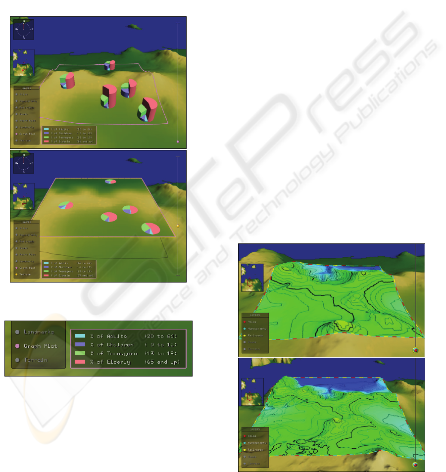
chart layer illustrated in figure 9 shows such a
hybrid chart layer. Classifications include both pie-
size and color. The semantics of the classifications
are available in an auxiliary attribute-classification
legend. This legend is a pop-up legend that is
visible when the chart layer is selected (figure 10).
One might argue that when the chart layer is
viewed in 3D, it offers an immediate impression of
the overall data with respect to the 3D spatial terrain
data. In the 2D mode it is more visually precise and
eliminates potential occlusions.
Figure 9: A transitioned chart layer employing a pie chart
view.
Figure 10: Auxiliary legend for pie chart classifications.
4.5 Zooming with the Layer System
A further addition to our hybrid GIS is a seamless
approach to camera zooming. This zooming feature
allows the expansion and contraction of the terrain
coverage, while maintaining a constant screen size
of the layer system interface. When zooming in and
out, the layers, control balls and slider, legend and
navigation tools all remain fixed in position and size
relative to the camera. The only aspects that
increase and decrease are the amount of terrain
covered by the layers.
In order to explain how this is implemented we
must consider how each layer is rendered. Each
layer’s geometry is essentially the same as the base
terrain itself. But, in addition to being (possibly)
flattened, the layer is clipped on four sides with four
clipping planes that are perpendicular to the layer.
Each clipping plane is the same distance from the
centre of the layer system but along four opposing
vectors. This ensures that we see a layer as a square
area of the grid rather than the entire terrain.
In order to zoom, while maintaining a fixed layer
size relative to the camera, we must simultaneously:
1) adjust the positions of the four clipping
planes surrounding the layers with respect to
the center of the layer system, and
2) move the camera backward or forwards along
the camera's line of sight.
For example, if we are zooming-out to see a larger
portion of the terrain, we must move all four
clipping plane outwards with respect to the center of
the layer system and simultaneously move the
camera backwards along its line of sight (figure 11).
The relative rates of movement of both the camera
and the four clipping planes must be precisely
coordinated in order to maintain the appearance of a
constant layer system size.
Figure 11: Zooming in (top) and out (bottom) on a layer
group.
VISUALIZING COLLAPSIBLE 3D DATA IN A HYBRID GIS
177

5 FUTURE DIRECTIONS
There remain many opportunities for extending the
system beyond its current form. One major
extension will involve the addition of advanced
query facilities. The integration of such querying
functionality will make our system broadly
applicable to a variety of tasks. The query results
will form new layers and will exhibit 3D icons and
labels. In order to provide such functionality we will
need to integrate 3D spatial data into a database
management system.
To complement the querying facilities we also
propose to add a data editing framework. It is also
our aim to undertake a usability study to confirm
that a hybrid system such as ours is advantageous to
the GIS community.
6 CONCLUSIONS
Our unique Geographical Information System
seamlessly integrates 2D and 3D views of the same
data. The system allows the user to view the 2D
data in direct relation to the 3D view within the
same view. By combining traditional 2D GIS with a
3D view we are able to take advantage of both types
of representations each with complementary
strengths. This is implemented as multiple layers of
information that are continuously transformed
between the 2D and 3D modes under the control of
the user, directly over the 3D base-terrain.
We propose that by providing a 2D-3D
transitional layer we can overcome both the self-
occlusion and terrain-occlusion issues. Our layering
system also offers a convenient means of handling
multiple heterogeneous sets of aspatial data under
user control. The system allows one to temporally
set aside data that is not currently relevant.
In this paper we have presented an array of
expanded capabilities for our distinctive hybrid GIS.
These additional facilities include: landmark layers,
chart layers, 3D point layers, layer grouping, unified
control of grouped layers, layer painting, and
zooming functionality.
ACKNOWLEDGEMENTS
This work was supported by an NSERC discovery
grant and a CFI New Opportunities Grant.
REFERENCES
Brooks, S., Whalley, J., 2005. A 2D/3D hybrid
geographical information system. In Proceedings of
ACM GRAPHITE, Dunedin, 323-330.
ESRI ArcGIS. (n.d.). Retrieved May 1, 2006, from
http://www.esri.com/software/arcgis/.
Hix, D., Hartson, H. R.,
1993. Developing User Interfaces:
Ensuring usability through product and process,
Wiley, New York.
Huang, B., Lin, H., 1999. GeoVR: a web-based tool for
virtual reality presentation from 2D data. In
Computers and Geosciences, 25, 1167-1175.
Kapler, T., Wright, W., 2005. Geo-time information
visualization. Information Visualization 4, 2, 136-146.
Köller, D., Lindstrom, P., Ribarsky, W., Hodges, L. F.,
Faust, N., Turner, G., 1995. Virtual GIS: A real-time
3D geographic information system. In Proceedings of
the IEEE Conference on Visualization '95, 94-100.
PAMAP GIS Topographer. (n.d.). Retrieved May 1, 2006,
from http://www.pigeomatics.com.
Reddy, M., Leclerc, Y., Iverson, L., Bletter, N., 1999.
TerraVisionII: Visualizing massive terrain databases
in VRML. In IEEE Computer Graphics and
Applications, 19, 2, 30-38.
Rishe, N., Sun, Y., Chekmasov, M., Andriy, S., Graham
S., 2004. System architecture for 3D terrafly online
GIS. In Proceedings of the IEEE Sixth International
Symposium on Multimedia Software Engineering
(MSE2004), 273-276.
Springmeyer, R. R., Blattner, M. M., Max, N. L., 1992. A
characterization of the scientific data analysis process.
In Proceedings IEEE Visualization, 235-242.
Stota, J., Zlatanova, S., 2003. 3D GIS, where are we
standing? In Workshop on Spatial, Temporal and
Multi-Dimensional Data Modeling and Analysis.
Tory, M., Swindells, C., 2003. Comparing ExoVis,
orientation icon, and in-place 3D visualization. In
Proceedings of Graphics Interface, 57-64.
Verbee, E. G., van Maren, R., Germs, F.J., Kraak, M.,
1999. Interaction in virtual views – linking 3D GIS
with VR. In International Journal of Geographics
Information Systems, 13, 4, 385-396.
Ware, C., Plumlee, M., Arsenault, R., Mayer, L. A.,
Smith, S., 2001. GeoZui3d: data fusion for interpreting
oceanographic data. In Proceedings of Oceans 2001,
3, 1960-1964.
Zlatanova, S., Rahman, A., Pilouk, M., 2002. Trends in
3D GIS development. Journal of Geospatial
Engineering, 4, 2, 1-10.
GRAPP 2007 - International Conference on Computer Graphics Theory and Applications
178