ON PROJECTION MATRIX IDENTIFICATION FOR CAMERA
CALIBRATION
Michał Tomaszewski and Władysław Skarbek
Institute of Radioelectronics, Warsaw University of Technology, Nowowiejska 15/19, 00-665 Warszawa, Poland
Keywords:
Projection matrix, homographic matrix, camera calibration, intrinsic parameters, Housholder symmetry.
Abstract:
The projection matrix identification problem is considered with application to calibration of intrinsic camera
parameters. Physical and orthogonal intrinsic camera models in context of 2D and 3D data are discussed. A
novel nonlinear goal function is proposed for homographic calibration method having the fast convergence of
Levenberg-Marquardt optimization procedure. Three models (linear, quadratic, and rational) and four opti-
mization procedures for their identification were compared wrt their time complexity, the projection accuracy,
and the intrinsic parameters accuracy. The analysis has been performed for both, the raw and the calibrated
pixel data, too. The recommended technique with the best performance in all used quality measures is the
Housholder QR decomposition for the linear least square method of the linear form of projection equations.
1 INTRODUCTION
Camera calibration is the fundamental generic prob-
lem in computer vision (Y. Ma, 2004). In case of
pinhole camera model, the problem usually refers to
estimation of camera intrinsic parameters K and to
camera pose R and camera locationC estimation with
respect to a selected coordinates frame. Both kinds
of parameters define, modulo constant factor, a pro-
jection matrix M which is the algebraic model in ho-
mogenous coordinates of the imaging geometry for
the given view of 3D or 2D scene:
p ≡ MP, p =


x
y
1


, P =



X
Y
Z
1



M = [M
3
,m
4
], M
3
∈ R
3×3
, m
4
∈ R
3
(1)
where projective relation ≡ makes equivalent all
points collocated in the same projective line. In al-
gebraic notation it means that for any P there exists
a scaling factor λ(P) for which the equation is true:
p = λ(P)MP.
The matrix K ∈ R
3×3
of intrinsic parameters de-
scribes the transformation from scene to camera pixel
coordinates on the projection plane. Since the choice
of coordinate axis for the camera is not unique the K
is not unique, too. However, the following decompo-
sition formula always holds:
M ≡ KR
−1
[I
3
,−C] (2)
where the pose matrix R = [r
x
,r
y
,r
z
] consists of the
camera frame axis defined by unit length vectors with
coordinates wrt the scene frame I
3
= [e
1
,e
2
,e
3
], and
C is the origin of the camera frame.
The matrix equivalence used in (2) is the equality
modulo constant factor: M
1
≡ M
2
if and only there
exists λ 6
= 0 such that M
2
= λM
1
.
Since any rotation in projection plane can be mod-
elled by the matrix R, the intrinsic matrix K is the
upper triangular matrix with positive elements on the
diagonal. In principle there are two approaches to
make the matrix K unique. In the most popular case,
the requirement of orthogonality R
t
R = I
3
makes by
QR decomposition of M
−1
3
, the unique selection of K
(O. Faugeras, 2001). We call this case of calibration
as orthogonal calibration and identify the fivefree pa-
rameters for the inverse matrix:
K
−1
o
=


k
1
k
2
k
3
0 k
4
k
5
0 0 1


(3)
92
Tomaszewski M. and Skarbek W. (2007).
ON PROJECTION MATRIX IDENTIFICATION FOR CAMERA CALIBRATION.
In Proceedings of the Second International Conference on Computer Vision Theory and Applications, pages 92-97
DOI: 10.5220/0002068000920097
Copyright
c
 SciTePress

In the less popular case, the requirement of orthog-
onality is replaced by the zero condition k
2
= 0. The
case is fully compliant with the physical model of pin-
hole camera having directly interpreted parameters:
K
p
=


f
x
0 c
x
0 f
y
c
y
0 0 1


(4)
where for pixel size s
x
×s
y
and focal length f we have
f
x
= f/s
x
, f
y
= f /s
y
, and (c
x
,c
y
) are pixel coordi-
nates of the image center, i.e. intersection point of
the projection plane by the camera z axis. Usually
c
x
≈ x
res
/2, c
y
≈ y
res
/2. Having the first two columns
u
x
, u
y
of M
−1
3
we get f
x
= 1/ku
x
k, f
y
= 1/ku
y
k.
In case of intrinsic calibration by 2D scene views
(less expensive and more accurate case) we have to
estimate the 2D version of M, i.e. the homographic
matrix H which relates planar points in the scene with
image pixels:
p ≡ HP, p =


x
y
1


, P =


X
Y
1


(5)
The relationship of the homographic projection H
with the intrinsic parameters is obtained from (2).
However now, the orthogonal calibration can be only
resolved from the homographic equation (5). Since
then Z = 0 and R
−1
= R
t
we have:
H = [h
1
,h
2
,h
3
] ≡ K
o
R
t
[e
1
,e
2
,−C]
K
−1
o
h
1
≡ e
1
, K
−1
o
h
2
≡ e
2
(6)
It implies the following two inherently nonlinear re-
lationships for K
o
and its vectorial representation
~
k =
[k
1
,...,k
5
]
t
:
h
t
1
K
−t
o
K
−1
o
h
2
= 0, h
t
1
K
−t
o
K
−1
o
h
1
= h
t
2
K
−t
o
K
−1
o
h
2
~
k
t
[h
◦t
1
h
◦
2
+ h
◦t
2
h
◦
1
]
~
k+ 2h
1
(3)h
2
(3) = 0
~
k
t
[h
◦t
1
h
◦
1
− h
◦t
2
h
◦
2
]
~
k+ h
2
1
(3) − h
2
2
(3) = 0
(7)
where for the vector h = [h(1),h(2),h(3)]
t
, a circle
operator assigns the following matrix:
h
◦
=

h(1) h(2) h(3) 0 0
0 0 0 h(2) h(3)

(8)
From the above introduction to camera calibration
problem we see that the accuracy of the projection
matrix M or H determined from 3D or 2D noisy data,
is of utmost importance.
In the presented research three models (linear,
quadratic, and rational) and four optimization proce-
dures for their identification were compared wrt their
time complexity, the projection accuracy, and the in-
trinsic parameters accuracy. The analysis has been
performed for both, the raw and the calibrated pixel
data, too.
2 MODELS FOR PROJECTION
IDENTIFICATION
Using Kronecker’s operation ⊗, the generic projec-
tion relation (1) can be transformed into the equation:
p = λ(P)MP = [I
3
⊗ P
t
]

~m
1

(9)
where the matrix M = [m
ij
], with m
34
= 1, has the
row-wise vectorial form
~m = [m
11
,m
12
,...m
21
,m
22
,...,m
31
,m
32
,m
33
]
t
It will be convenient to separate the matrix opera-
tor A(P) = I
3
⊗ P
t
into three row vector operators
A
1
,A
2
,A
3
:
A(P) = I
3
⊗ P
t
=


A
1
(P) 0
A
2
(P) 0
A
3
(P) 1


(10)
It is easy to check that the same separation is true
for the homographic matrix H = [h
ij
] for which the
vectorial form
~
h has 8 elements:
~
h = [h
11
,h
12
,h
13
,h
21
,h
22
,h
23
,h
31
,h
32
]
t
2.1 Rational Model
The most close model to the projective equation (9)
is the nonlinear model wrt ~m having the form of two
rational functions:
E
x
(~m;P) =
A
1
(P)~m
A
3
(P)~m+1
− x
E
y
(~m;P) =
A
2
(P)~m
A
3
(P)~m+1
− y
(11)
In order to find the projection matrix, for the spa-
tial non-planar points P
i
projected onto image pixels
p
i
, i = 1,...,n
p
(n
p
≥ 6) we optimize by Levenberg-
Marquardt method, the followingnonlinear goal func-
tion:
N (~m) =
n
p
∑
i=1

E
2
x
(~m;P
i
) + E
2
y
(~m;P
i
)

The Jacobian matrix J, required by this procedure, has
the compact form:
J(~m;P) =




A
1
(P)
A
3
(P)~m+1
−
A
1
(P)~mA
3
(P)
(A
3
(P)~m+1)
2
A
2
(P)
A
3
(P)~m+1
−
A
2
(P)~mA
3
(P)
(A
3
(P)~m+1)
2




(12)
It is interesting that the formulas (11), (12) are also
valid for the homographic matrix H with ~m replaced
by
~
h and P
t
= [X,Y,Z,1] replaced by P
t
= [X,Y,1].
ON PROJECTION MATRIX IDENTIFICATION FOR CAMERA CALIBRATION
93

2.2 Linear Model
The roots of rational functions (11) are also the solu-
tions of the following linear system of equations:
A(P, p)~m =

A
1
(P) − xA
3
(P)
A
2
(P) − yA
3
(P)

~m =

x
y

(13)
Considering n
p
spatial points P
i
and their images
p
i
, i = 1, . . . , n
p
we get 2n
p
linear equations A~m ≃ b
defined by the matrix A and the right hand side vector:
A =



A(P
1
, p
1
)
.
.
.
A(P
n
p
, p
n
p
)



, b =



b(p
1
)
.
.
.
b(p
n
p
)



The same construction is valid for the homographic
matrix H.
There are many techniques finding efficiently the
minimum solution ~m
∗
of the linear least square prob-
lem A~m ≃ b for the following goal function:
L(~m) = kA~m− bk
2
=
n
p
∑
i=1
kA(P, p) − b(p)k2.
The most popular method is the pseudo-inverse ma-
trix A
+
method (R. Klette, 1996) which is found using
SVD decomposition for A = UΣV
t
:
A
+
= VΣ
+
U
t
where the diagonal matrix Σ
+
is the pseudo-inverseof
the diagonal matrix Σ :
Σ = diag(σ
1
,...,σ
r
,0,... , 0)
Σ
+
= diag(1/σ
1
,...,1/σ
r
,0,... , 0)
where r isthe rank of A. Then the least square solution
is given by the formula
~m
∗
= A
+
b
Let r = 11 for 3D case and r = 8 for 2D case. The
faster algorithm for the case when r < 2n
p
is R-SVD
algorithm. Using the complexity formulas for SVD
from (G. Golub, 1989) we have the following number
of flops for the pseudo-inverse method:
FLOPS
PINV
(n
p
,r) = 6n
p
r(8r/3 + 1) + 20r
3
(14)
Another technique finding the optimal solution is
based on triangulation of matrix A by Housholder’s
symmetries H
a
i
, i = 1,. . . , r. The process is part of
QR decomposition. However we need only the tri-
angular form T
H
and concurrently transformed right
hand side b
H
. Then the least square solution is given
by the formula:
~m
∗
= T
−1
H
b
H
The exact count of flops for HS-QR approach gives
the formula:
FLOPS
HS
(n
p
,r) = 6n
p
r(r+1)+r
2
(−r/2+3+5/(2r))
The difference of the measures shows the computa-
tional advantage of HS-QR approach.
FLOPS
PINV
(n
p
,r) − FLOPS
HS
(n
p
,r) =
= 10n
p
r
2
+ 41r
3
/2− 3r
2
− 5r/2
For 3D case, r = 11 and then
FLOPS
PINV
(n
p
,11) − FLOPS
HS
(n
p
,11) >
1210n
p
+ 25000.
While in 2D case, r = 8 and the flops difference has
the formula:
FLOPS
PINV
(n
p
,8) − FLOPS
HS
(n
p
,8) >
> 640n
p
+ 10000.
2.3 Quadratic Model
In the literature referring to camera calibration prob-
lems the quadratic model is frequently recommended
(Y. Ma, 2004). It is obtained from (13) by aggregation
of quadratic errors produced by each pair P
i
, p
i
.
Let
~
m
′
extends ~m by m
3,4
. Then, the error of repro-
ducing p from P is described by the following matrix
B(P, p) :
B(P, p)
~
m
′
=

A
1
(P) − xA
3
(P) −x
A
2
(P) − yA
3
(P) −y

~
m
′
≃

0
0

The same form of error matrix we obtain for 2D case
extending
~
h by h
3,3
.
The total squared error leads to the quadratic form
defined by the matrix B :
L
′
(
~
m
′
) =
∑
n
p
i=1
kB(P
i
, p
i
)
~
m
′
k
2
=
=
∑
n
p
i=1
~
m
′
t
B
t
(P
i
, p
i
)B(P
i
, p
i
)
~
m
′
=
=
~
m
′
t

∑
n
p
i=1
B
t
(P
i
, p
i
)B(P
i
, p
i
)

~
m
′
=
~
m
′
t
B
~
m
′
The minimization of L
′
(
~
m
′
) is obtained from
SVD: B = UΣV
t
. Namely, from the singular base
U
r
= [u
1
,...,u
r+1
], we take the vector u
r+1
and con-
vert to matrix form.
The computational complexity for the quadratic
method has the formula:
FLOPS
SVD
(n
p
,r) = 4n
2
p
(r+ 1)
2
+ 17(r+ 1)
3
.
Since the above formula is quadratic in n
p
, the com-
putational advantage of HS-QR method over SVD is
also quadratic. It follows from computational over-
head to get the matrix B. We could avoid this by ap-
plying SVD to the global error matrix:

B(P
1
, p
n
),...,B(P
n
p
, p
n
p
)

t
.
However, then we get a procedure equivalent to
pseudo-inverse method with complexity linearly in-
ferior in n
p
to HS-QR approach.
VISAPP 2007 - International Conference on Computer Vision Theory and Applications
94

3 INTRINSIC CALIBRATION
We have investigated this problem for both, the or-
thogonal and physical calibration cases, detailed in
the introduction.
3.1 3D Calibration Scene
In 3D case when pixel data is obtained from images of
calibration cube we start from identification of physi-
cal model.
The image center is roughly estimated from the
camera image resolution and its location is accurately
estimated during the lens distortion modelling. It
is interesting that the remaining physical parameters
f
x
, f
y
have simple formulas if M
3
is already estimated.
Namely, if M
−1
3
= [u
x
,u
y
,u
z
] then
M
−1
3
= [u
x
,u
y
,u
z
] = RK
−1
p
=
= [r
x
,r
y
,r
z
]


1/ f
x
0 −c
x
/ f
x
0 1/ f
y
−c
y
/ f
y
0 0 1


(15)
Hence
f
x
=
1
ku
x
k
, f
y
=
1
ku
y
k
, r
x
= f
x
u
x
, r
y
= f
y
u
y
r
z
=
u
z
+c
x
u
x
+c
y
u
y
ku
z
+c
x
u
x
+c
y
u
y
k
(16)
Having parameters f
x
, f
y
,c
x
,c
y
, the calibration
matrix K
p
is identified according (4). The matrix K
o
can be found from the matrix K
p
by closed form for-
mulas. However, we have found that QR procedure
applied to M
3
:
M
−1
3
QR
= RK
−1
o
gives K
o
entries more accurate when data is noisy.
3.2 2D Calibration Scene
In 2D case when calibration is performed from homo-
graphic matrices obtained on the basis of chessboard
images the error function is based on relationships (7)
applied to j-th view, j = 1,...,n
v
:
E
( j)
1
(
~
k) =
~
k
t
A
j
~
k+ 2h
( j)
1
(3)h
( j)
2
(3)
E
( j)
2
(
~
k) =
~
k
t
B
j
~
k+ (h
( j)
1
)
2
(3) − (h
( j)
2
)
2
(3)
(17)
where the symmetric matrices A
j
, B
j
are defined as
follows
A
j
= (h
( j)
1
)
◦t
(h
( j)
2
)
◦
+ (h
( j)
2
)
◦t
(h
( j)
1
)
◦
B
j
= (h
( j)
1
)
◦t
(h
( j)
1
)
◦
− (h
( j)
2
)
◦t
(h
( j)
2
)
◦
In order to find the calibration matrix K
o
repre-
sented by the vector
~
k, we optimize by Levenberg-
Marquardt method, the followingnonlinear goal func-
tion:
N
K
(~m) =
n
v
∑
j=1
h
(E
( j)
1
)
2
(
~
k) + (E
( j)
2
)
2
(
~
k)
i
The Jacobian matrix J, required by this procedure, has
a simple form for j = 1,...,n
v
:
J
( j)
(
~
k) = 2
"
~
k
t
A
j
~
k
t
B
j
#
(18)
Having intrinsics in orthogonal model
~
k we can
get easily the missing parameters for the physical
model:
f
x
=
1
k
1
, f
y
=
1
q
k
2
2
+ k
2
4
0.0 0.5 1.0 1.5 2.0 2.5 3.0
0.0
0.5
1.0
1.5
2.0
2.5
3.0
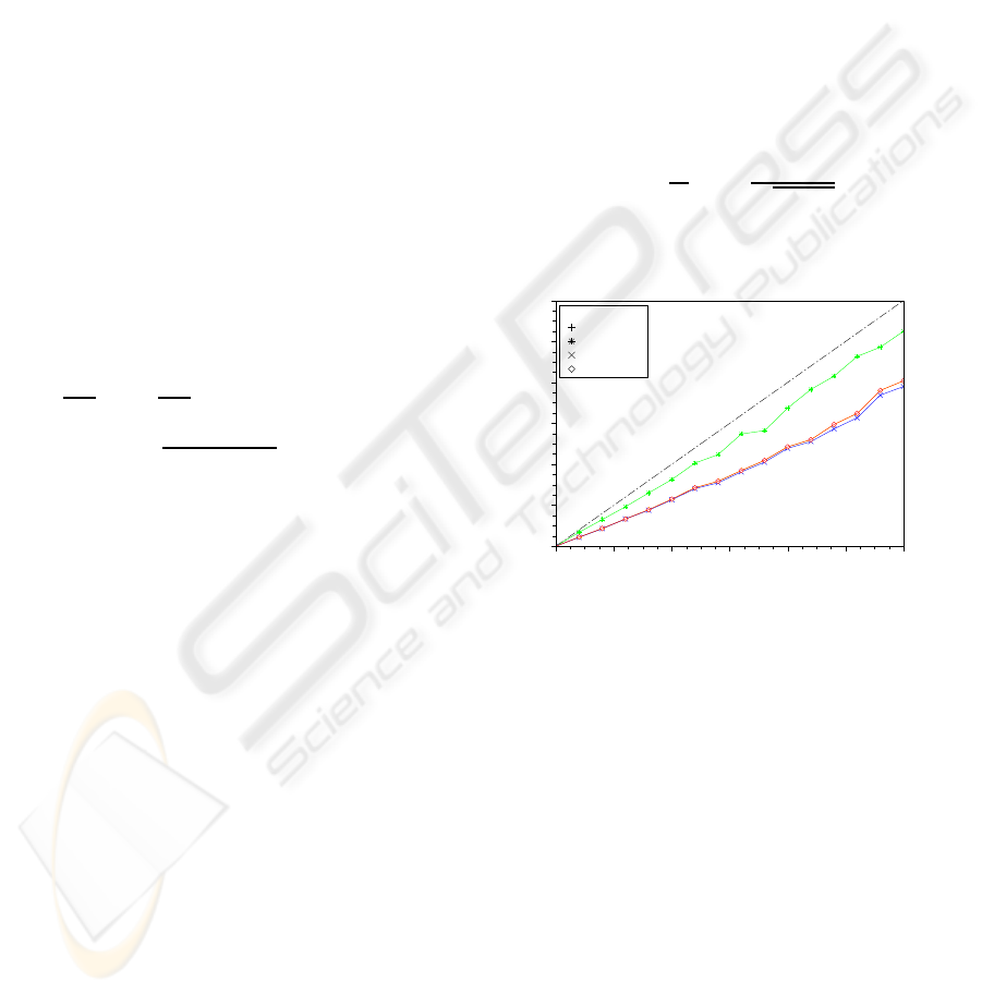
Projection Error for Uniform Noise
Average Noise for Input Pixels
Average Error of Projection in Pixels
y=x
linear: PINV
quadratic: SVD
nonlinear: NLSM
linear: HS−QR
Figure 1: The average projection error for matrix identi-
fied from noisy pixels. The noise is uniform in the interval
[−σ,+σ], σ ∈ [0,3] is measured in pixels.
4 EXPERIMENTS
We have conducted our experiments on both, the real
and the synthetic data. Real pixel data has been
mainly located manually. In case of optical distortion
modelling, where thousands of corners in calibration
grid are required, their coordinates were detected au-
tomatically by our computer program.
For the identification of the projection matrix M
and the homographic matrix H four models were
compared: linear by PINV, quadratic by SVD, non-
linear by LM, and linear by HS-QR.
The accuracy of matrix identification was mea-
sured directly by Frobenius distance to the ground-
truth matrix and indirectly by the average displace-
ment of pixels projected by the identified matrix from
ON PROJECTION MATRIX IDENTIFICATION FOR CAMERA CALIBRATION
95

noisy data wrt to pixels projected by the ground truth
matrix.
In Figures 1, 2 we present comparative results
of projection accuracy for the four analyzed models
under uniform and normal input noise and with and
without pixel normalization operation. The pixel nor-
malization is guided by the physical intrinsic parame-
ters
p
′
= K
−1
p
p, x
′
= (x− c
x
)/ f
x
, y
′
= (y− c
y
)/ f
y
.
The similar normalization operation is used before the
calibration of extrinsic parameters (Hartley, 1997).
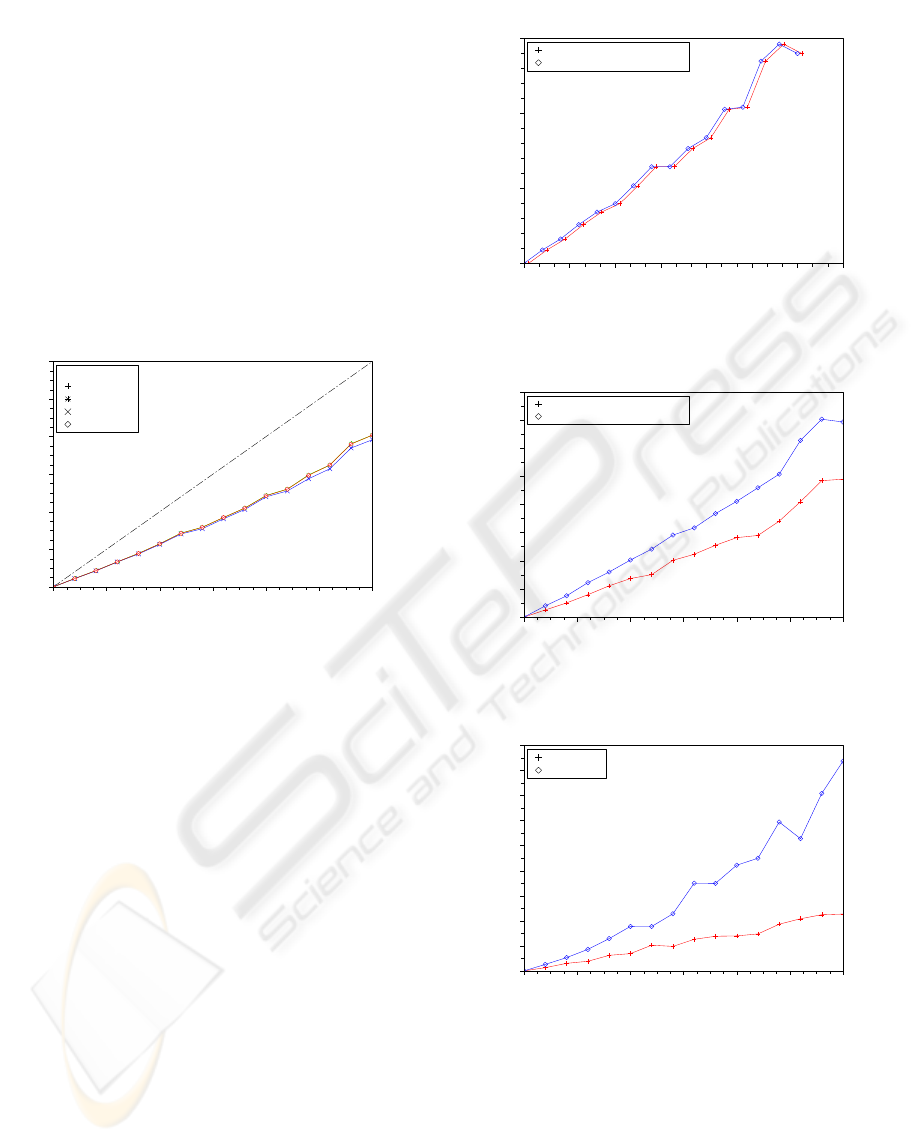
0.0 0.5 1.0 1.5 2.0 2.5 3.0
0.0
0.5
1.0
1.5
2.0
2.5
3.0
Projection Error for Uniform Noise and Normalized Pixels
Average Noise for Input Pixels
Average Error of Projection in Pixels
y=x
linear: PINV
quadratic: SVD
nonlinear: NLSM
linear: HS−QR
Figure 2: The average projection error for matrix identified
from noisy pixels. The noise is uniform in [−σ,+σ] and
σ ∈ [0, 3] is measured in pixels. The pixel normalization is
used.
We see from Figure 1 that PINV, HS-QR, and ML
(initialized by PINV) have comparable accuracy (with
slight advantage of nonlinear model) while SVD has
significantly higher projection error. When pixel nor-
malization is applied (in practice not always possi-
ble!) then all the methods transform input pixel noise
into output noise in the same way scaling it down (cf.
Figure 2) by a factor of two. The similar behavior has
been observed for normal noise.
Figures 3, 4 illustrate the dependence of absolute
projection matrix and intrinsic matrix (3D case) er-
rors (per matrix element) on input pixel noise. While
the relationship for projection matrix is exactly the
same (the graphs were slightly shifted to distinguish
them) for independently whether we use in calibra-
tion physical or orthogonal model, the accuracy of el-
ement identification for the physical intrinsic model is
higher than for the orthogonal intrinsic model.
Calibration of intrinsic parameters from homogra-
phies wrt the selected computational model is ana-
lyzed in Figures 5, 6, and 7.
The advantage of linear over quadratic model is
observed on all these graphs.
0.0 0.5 1.0 1.5 2.0 2.5 3.0 3.5
0.00
0.05
0.10
0.15
Projection Matrix Error on Pixel Noise
Average Noise for Input Pixels
Average Projection Matrix Error
physical calibration model for intrinsics
orthogonal calibration model for intrinsics
Figure 3: Average projection matrix absolute error identi-
fied from noisy pixels.
0.0 0.5 1.0 1.5 2.0 2.5 3.0
0.0
0.5
1.0
1.5
2.0
2.5
3.0
3.5
4.0
Intrinsics Matrix Error on Pixel Noise
Average Noise for Input Pixels
Average Intrinsics Matrix Error
physical calibration model for intrinsics
orthogonal calibration model for intrinsics
Figure 4: Average intrinsic matrix absolute error identified
from noisy pixels.
0.0 0.5 1.0 1.5 2.0 2.5 3.0
0.000
0.005
0.010
0.015
0.020
0.025
0.030
0.035
0.040
0.045
Physical Intrinsics Matrix Error on Pixel Noise
Average Noise for Input Pixels
Average Physical Intrinsics Matrix Error
linear model
quadratic model
Figure 5: Average physical intrinsics matrix error for pixel
noise.
In the screen shot below we have the results of in-
trinsic calibration for real data extracted from 16 im-
ages of chessboard.
VISAPP 2007 - International Conference on Computer Vision Theory and Applications
96

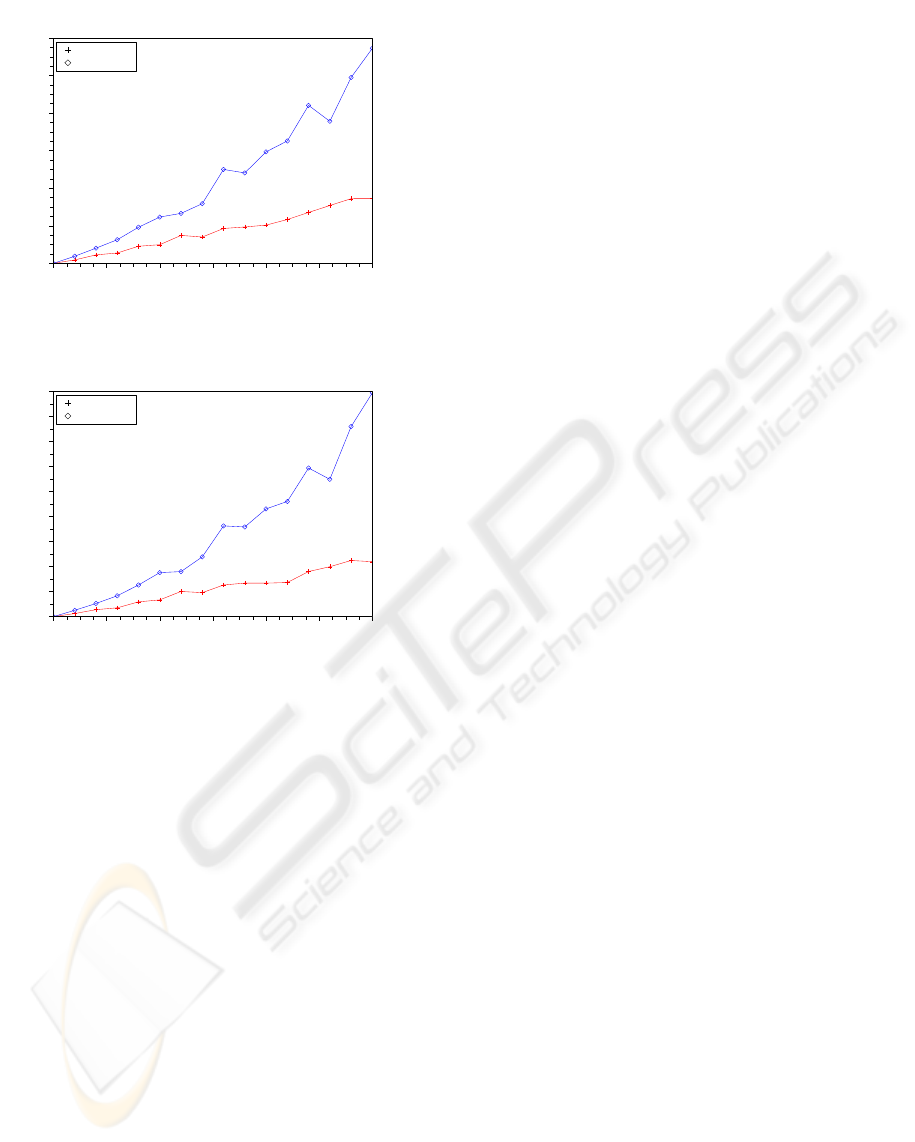
0.0 0.5 1.0 1.5 2.0 2.5 3.0
0.00
0.01
0.02
0.03
0.04
0.05
0.06
Orthogonal Intrinsics Matrix Error on Pixel Noise
Average Noise for Input Pixels
Average Orthogonal Intrinsics Matrix Error
linear model
quadratic model
Figure 6: Average orthogonal intrinsics matrix error for
pixel noise.
0.0 0.5 1.0 1.5 2.0 2.5 3.0
0.000
0.005
0.010
0.015
0.020
0.025
0.030
0.035
0.040
0.045
Focus by Pixel Width Error on Pixel Noise
Average Noise for Input Pixels
Average Focus by Pixel Width Error
linear model
quadratic model
Figure 7: Average focus to pixel width error for pixel noise.
-->[Kp,Ko]=realKpKoByHomographies(3073/2,2305/2)
Ko =
2463.0976 3.2421405 1535.4054
0. 2473.6315 1142.4508
0. 0. 1.
Kp =
2463.0976 0. 1536.5
0. 2473.6294 1152.5
0. 0. 1.
5 CONCLUSION
The projection matrix identification problem is con-
sidered with application to calibration of intrinsic
camera parameters.
Physical and orthogonal intrinsic camera models
in context of 2D and 3D data are discussed.
A novel nonlinear goal function is proposed for
homographic calibration method having the fast con-
vergence of Levenberg-Marquardt optimization pro-
cedure.
Three models (linear, quadratic, and rational) and
four optimization procedures for their identification
were compared wrt their time complexity, the projec-
tion accuracy, and the intrinsic parameters accuracy.
The analysis has been performed for both, the raw
and the calibrated pixel data, too.
The recommended technique with the best perfor-
mance in all used quality measures is the Housholder
QR decomposition for the linear least square method
of the linear form of projection equations.
REFERENCES
G. Golub, C. L. (1989). Matrix Computations. The Johns
Hopkins University Press, Baltimore and London, 2nd
edition.
Hartley, R. (1997). In defence of the eight-point algorithm.
IEEE Transcations on Pattern Analysis and Machine
Intelligence, 19(6):580–593.
O. Faugeras, Q. L. (2001). Geometry of Multiple Images.
The MIT Press, Cambridge, Massachusetts.
R. Klette, K. Schluns, A. K. (1996). Computer Vision -
Three-Dimensional Data From Images. Springer, Sin-
gapore.
Y. Ma, S. Soatto, e. a. (2004). An Invitation to 3-D Vision.
Springer, Cambridge, Massachusetts.
ON PROJECTION MATRIX IDENTIFICATION FOR CAMERA CALIBRATION
97