NEW ADAPTIVE ALGORITHMS FOR OPTIMAL FEATURE

EXTRACTION FROM GAUSSIAN DATA

Youness Aliyari Ghassabeh and Hamid Abrishami Moghaddam

Electrical Engineering Department, K .N. Toosi University of Technology, Tehran, Iran

Keywords: Adaptive learning algorithms, Feature extraction, Covariance matrix, Gaussian data.

Abstract: In this paper, we present new adaptive learning algorithms to extract optimal features from

multidimensional Gaussian data while preserving class separability. For this purpose, we introduce new

adaptive algorithms for the computation of the square root of the inverse covariance matrix

21−

. We

prove the convergence of the adaptive algorithms by introducing the related cost function and discussing

about its properties and initial conditions. Adaptive nature of the new feature extraction method makes it

appropriate for on-line signal processing and pattern recognition applications. Experimental results using

two-class multidimensional Gaussian data demonstrated the effectiveness of the new adaptive feature

extraction method.

1 INTRODUCTION

Feature extraction is generally considered as a

process of mapping the original measurements into a

more effective feature space. When we have two or

more classes, feature extraction consists of choosing

those features which are the most effective for

preserving class separability in addition to

dimension reduction (Theodoridis, 2003). One of the

most used techniques for this purpose is linear

discriminant analysis (LDA) algorithm. LDA

algorithm has been widely used in signal processing

and pattern recognition applications in which feature

extraction is inevitable, such as face and gesture

recognition and hyper-spectral image processing

(Chang and Ren, 2000; Chen et al., 2000;

Lu et al.

2003) Conventional LDA algorithm is used only in

off-line applications. However, the needs for

dimensionality reduction in real time applications

such as on-line face recognition, motivated

researchers to introduce adaptive versions of LDA.

Chaterjee and Roychowdhury presented an adaptive

algorithm and a self-organizing LDA network for

feature extraction from Gaussian data (Chatterjee

and Roychowdhury, 1997). They introduced an

adaptive method for computation of

21−

in which

is the symmetric positive definite scattering

matrix of a random vector sequence. However, they

didn’t introduce any cost function related to their

adaptive algorithm. Therefore, they used the

stochastic approximation theory in order to prove the

convergence of their adaptive equation and outlined

networks for feature extraction. On the other hand,

the approach presented in (Chatterjee and

Roychowdhury, 1997) suffers from low convergence

rate. Recently, Abrishami Moghaddam et al. (2003;

2005) proposed three new adaptive methods based

on steepest descent, conjugate direction and

Newton-Raphson optimization techniques to hasten

convergence of the adaptive algorithm.

In this study, we present new adaptive algorithms

for the computation of

21−

. Furthermore, we

introduce a cost function related to these algorithms

and prove their convergence by discussing about the

properties and initial conditions of this cost function.

Existence of the cost function and its

differentiability facilitate the convergence analysis

of the new adaptive algorithms without using

complicated stochastic approximation theory. We

will show effectiveness of these new adaptive

algorithms for extracting optimal features from two-

class multi-dimensional Gaussian sequences.

The organization of the paper is as follows. The

next section describes the fundamentals of optimal

feature extraction from Gaussian data. Section 3,

presents the new adaptive equations and analyzes

their convergence by introducing the related cost

function and discussing about initial conditions.

Section 4, is devoted to simulations and

182

Aliyari Ghassabeh Y. and Abrishami Moghaddam H. (2007).

NEW ADAPTIVE ALGORITHMS FOR OPTIMAL FEATURE EXTRACTION FROM GAUSSIAN DATA.

In Proceedings of the Second International Conference on Computer Vision Theory and Applications, pages 182-187

DOI: 10.5220/0002067501820187

 SciTePress

experimental results. Finally, concluding remarks

are given in section 5.

2 OPTIMAL FEATURES FOR

GAUSSIAN DATA

Let

},...,,{

21 L

be the L classes in which our

patterns belong and

ℜ∈x

be a pattern vector

whose mixture distribution is given by

)(xp

. In a

sequel, it is assumed that a priori

probabilities

LiP

,...,1,)( =

, are known. If they

are not explicitly known, they can easily be

estimated from the available training vectors. For

example, if N is the total number of available

training patterns and N

(i=1,…,L) of them belong

, then

NN)(P

≈ω

. Consider conditional

probability densities

Lip

,...1,)|( =

and

posterior probabilities

LiP

,...1, )( =x

are known.

Using Bayes classification rule, we can state that the

pattern

is classified to

ijandLjiPP

≠

> ,...,1,,)|()|( xx

In other words, the L a posteriori probability

functions, mentioned above, are sufficient statistics,

and carry all information for classification in the

Bayes sense. The Bayes classifier in this feature

space is a piecewise bisector classifier which is its

simplest form (Fukunaga, 1990). Gaussian

distribution in general has a density function in the

following form

where the distance function

)(

, is defined by:

Which

ℜ∈x is a random vector,

is a

symmetric covariance matrix and

is a

vector

denoted mean value of the random sequence.

Considering the feature:

)(pln)(Pln)|(pln)|(Pln

iii

xxx −ω

ω=ω

(3)

for class

, i=1,…L, it will appear that,

)|( ln

is the relevant feature for class

(recalling that in feature extraction, additive and

multiplicative constants do not modify the subspace

onto which the distributions are mapped). Supposing

unimodal Gaussian distribution, the feature

)|( ln

reduces to a quadratic function

)(x

defined as:

Lif

,...1 , )()()(

=−−=

−

mxΣmxx

(4)

where

and

are the class

’s mean value

and covariance matrix, respectively. The

function

)(x

, can be expressed in the form of a

norm function ( Fukunaga, 1990) :

Lif

iii

,...,1,||)(||)(

=−=

−

mxΣx

(5)

From the above discussion, it is clear that

function

)(x

is the sufficient information for

classification of Gaussian data with minimum Bayes

error. In other words, after computation of

)(x

for

i=1 …,L, it is easy to decide about classification of

the unknown vector

. Generally speaking, in on-

line applications, the values of

21−

and

are

unknown. Therefore, we should find a rule for

adaptive estimation of these values and

compute

)(x

. In the next section, a new method for

adaptive computation of

21−

will be presented.

In addition, we introduce a cost function related to

this adaptive equation, and use it for proving its

convergence.

3 ADAPTIVE COMPUTATION

21−

AND

CONVERGENCE PROOF

We define the cost function

)(wJ

with

parameter

ℜ→ℜ

×nn

J :

as follows:

)(

xxW

W tr

−=

(6)

)(wJ

, is a continuous function with respect to

The expected value of J (for constant

) is given

by:

)(

))((

ΣW

W tr

JE −=

(7)

where

is the covariance matrix. The first

derivative of E(J) is computed as follows (assuming

that

is a symmetric matrix) (Magnus, Neudecker,

1999):

IΣWWWΣΣW

−++=

∂

3) (

))((

(8)

)(

||)2(

),(

Σm

−

(1)

)()()(

mxΣmxx −−=

−t

(2)

NEW ADAPTIVE ALGORITHMS FOR EXTRACTING OPTIMAL FEATURES FROM GAUSSIAN DATA

183

The unique zero solution of (8) is

21−

, the

second derivative of the expected value of the cost

function is equal to (Magnus, Neudecker, 1999):

WΣΣWIΣWΣWI

⊗+⊗+⊗+⊗=

∂

)(2)(2

))((

(9)

In (9) it is assumed that

is a symmetric matrix

that it commutes with

. If we substitute

in (9)

with

21−

, the answer will be:

21212121

ΣW

ΣΣΣΣIΣΣI

−−

⊗+⊗+⊗+⊗

∂

−

)(2)(2

))(J(E

(10)

where (10) is a positive definite matrix. From the

above discussion, it can be concluded that the cost

function

)(wJ

has a minimum that occurs at

21−

(Magnus, Neudecker, 1999). Using the gradient

descent optimization method (Widrow, Stearns,

1985; Hagan, Demuth, 2002), we obtain the

following adaptive equation for the computation

21−

)3)((

)

)(

(

111111

kkk

kkkk

WxxWxxWxxW

++++++

++−

∂

−+=

(11)

In (11),

1+k

is the estimation of

21−

in k+1-

th iteration.

is the step size and

1+k

x is the input

vector at iteration k+1. Equation (11) updates the

estimation of

21−

, using the last estimation and

the present input vector. The only constraint on (11)

is its initial condition. That means

must be a

symmetric and positive definite matrix

satisfying

ΣWΣW =

. It is quite easy to prove that if

is a symmetric and positive definite matrix, then

all values of

( i=2,3,…) will be symmetric and

positive definite. Therefore, the final estimation also

will have these properties (which are essential for

covariance matrix). To avoid confusion for choosing

the initial value

, we considered

equal to

identity matrix multiplied by a positive constant

(

=αI).

According to the result reported by (Kushner,

Clarck, 1978; Benveniste, Metivier, 1990), the

stochastic gradient algorithm in the form of:

),(

11 ++

−=

kkkkk

(12)

where f(θ,y)=grad

F(θ,y) and (Y

)

k>0

are

independent identically distributed

ℜ

-valued

random variables, converges almost surely towards a

solution of the minimization problem: min

E (F

(θ,Y)). As indicated in (12), in order to minimize E

(F (θ,Y)), the stochastic gradient algorithm uses the

random variable f(θ,Y) instead of its expectation in

the ordinary gradient method. The above argument

is another approach for proving the convergence of

(11) towards

21−

It is easy to show that if

considered a

symmetric and positive definite matrix which satisfy

ΣWΣW

then expected value of (11) will be equal

to the following equations:

Therefore (11) is simplified to three more

efficient forms as follows:

)(

kkkkkk +++

−+= xxWIWW

(14)

)(

kkkkkk +++

−+= xxWIWW

(15)

)(

111 k

kkkkkk

WxxWIWW

+++

−+=

(16)

Existence of the cost function for the new

adaptive

21−

algorithms has the following

advantages compared to the former one (Chatterjee

and Roychowdhury, 1997): i) it simplifies the task

for proving the convergence; ii) it helps to evaluate

the accuracy of the current solutions. For example,

in the cases of different initial conditions and

various learning rates, one is enable to evaluate

which initial condition and learning rate outperform

others. Furthermore, the former adaptive equation in

(Chatterjee and Roychowdhury, 1997) uses a fix or

monotonically decreasing learning rate which results

in low convergence speed, but introducing a cost

function related to the adaptive algorithm make it

possible to determine the learning rate efficiently in

every stage in order to increase the convergence rate.

There are different methods for adaptive

estimation of the mean vector. The following

equation was used in (Chatterjee and

Roychowdhury, 1997; Abrishami Moghaddam et al.,

2003; 2005):

)(

11 kkkkk

mxmm −

(17)

where η

satisfies Ljung assumptions ( Ljung ,

1977) for the step size. Alternatively, one may use

the following equation (Ozawa et al., 2005; Pang et

al., 2005):

)(

) (

)()(E

kkkk

kk1k

ΣWIW

WΣWIW

ΣWIWW

−η+=

(13)

VISAPP 2007 - International Conference on Computer Vision Theory and Applications

184

(18)

For the experiments reported in the next section,

we used (17) in order to estimate the mean value in

each iteration.

4 SIMULATION RESULTS

In this section, we used on of the (14-16) described

in the previous section to estimate

21−

and

extracted features from Gaussian data for

classification

4.1 Experiments on

21−

Algorithm

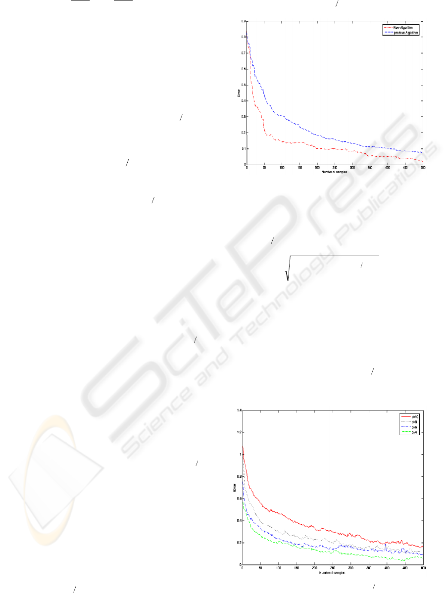
In the first experiment, we compared the

convergence of the new adaptive

21−

algorithm

with the algorithm proposed in (Chatterjee and

Roychowdhury, 1997). We used the first covariance

matrix in (Okada and Tomita, 1985), which is a

1010 ×

covariance matrix and multiplied it, by 20

(Figure 1). The ten eigenvalues of this matrix in

descending order are 117.996, 55.644, 34.175,

7.873, 5.878, 1.743, 1.423, 1.213 and 1.007. Figure

2 compares the error of each algorithm as a function

of sample number. As illustrated, the new algorithm

can converges with an accelerated rate than the

previous algorithm. We also compared the

convergence rate of the new adaptive

21−

algorithm in 4, 6, 8 and 10 dimensional spaces.

⎥

⎦

⎤

⎢

⎣

⎡

−−−

−−−−

−−−−−−

−−

−−−

−−

−

=Σ

341.0015.0028.0120.0095.0003.0003.0030.0065.0032.0

067.0078.0011.0005.0008.0001.0041.

0031.0002.0

450.1343.0248.0069.0022.0298.0057.0030.0

750.2544.0058.0042.0038.0154.00155

720.5088.0016.0450.0367.0136.0

071.0005.0055.0011.0010.0

084.0017.0028.0005.0

430.1018.0

053.0

373.0038.0

091.0

Figure 1: Sample covariance matrix used in

21−

experiments.

We used the same covariance matrix as in the

first experiment for generating 10 dimensional data

and three other matrices were selected as the

principal minors of that matrix.

In all experiments, we chose the initial value

equal to identity matrix multiplied by 0.6, and then

using a sequence of Gaussian input data (training

data) estimated

21−

. For each covariance matrix,

we generated 500 samples of zero-mean Gaussian

data and estimated the

21−

matrix using (14).

Figure 2: Comparison of convergence rate between new

algorithm and previous algorithm.

For each experiment, at k-th iteration, we

computed the error e(k) between the estimated and

actual

21−

matrices by:

∑∑

−

−=

actualij

kke

221

))(()( ΣW

(19)

For each covariance matrix, we computed the

norm of error in every iteration. Figure 3 shows

values of the error during iterations for each

covariance matrix. The final values of error after 500

samples are error=0.169 for d=10, error=0.118 for

d=8, error=0.102 for d=6 and error=0.0705 for d=4.

As expected, the simulation results confirmed the

convergence of (14) toward the

21−

. We repeated

the same experiment using (15) and (16) and

obtained similar results.

Figure 3: Convergence of the

21−

algorithm for

different covariance matrices.

NEW ADAPTIVE ALGORITHMS FOR EXTRACTING OPTIMAL FEATURES FROM GAUSSIAN DATA

185

4.2 Extracting Optimal Features from

Two Class Gaussian Data

As discussed in section 2, it is apparent that for

Gaussian data, the feature

)(x

is equal

221

||)(||

mxΣ −

−

, using (14-16), (17) and the

training sample sequence, we estimated

21−

and

For each training data belong to

we updated

first

21−

using (14-16) and then refreshed

applying (17), finally, we computed the norm

)(

mxΣ −

−

. After computation of the mean

value and

21−

according to (5), it is possible to

classify the next coming Gaussian data. At the end

of this process, we compute the number of

misclassifications. For testing the effectiveness of

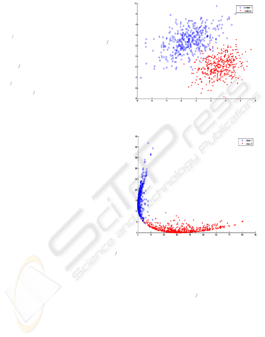
(14-16) in the case of two class Gaussian data, we

generated 500 samples of 2 dimensional Gaussian

data; each sample belonged to one of two classes

with different covariance matrices and mean vectors.

For each pattern

, we extracted features

)(

and

)(

. According to these optimal

features, we transformed incoming Gaussian data

into optimal feature space. Figures 4 and 5 show the

comparison between samples in the original space

and transformed samples in the optimal feature

space. Two Gaussian classes

and

had the

following parameters:

⎥

⎦

⎤

⎢

⎣

⎡

⎥

⎦

⎤

⎢

⎣

⎡

−

⎥

⎦

⎤

⎢

⎣

⎡

⎥

⎦

⎤

⎢

⎣

⎡

−

2211

QmQm

Figure 4 shows the distribution of samples from

two classes. It is obvious that two classes are not

linearly distinguishable. After estimation of

21−

by (14-16) and estimation of

by (17), we are

able to extract f

and f

from the training data.

Figure 5 shows the transformed data in optimal

feature space. It is apparent from Figure 5 that two

Gaussian classes are linearly separable in the

optimal feature space. In other words, in the optimal

feature space, we can draw a straight line to separate

two classes However, in their original space; two

classes are overlapped and are not linearly separable.

By extracting optimal features, only 9 sample data

among 1000 total sample, were misclassified by a

linear classifier.

Figure 4: Distribution of two class Gaussian data in the

original space.

Figure 5: Distribution of two class Gaussian data in the

optimal feature space.

5 CONCLUSIONS

In this paper, we presented new adaptive algorithms

for computation of

21−

and introduced a cost

function related to them. We proved the

convergence of the proposed algorithms using the

continuity and initial conditions of the cost function.

Simulation results on two class Gaussian data

demonstrated the performance of the proposed

algorithms for extracting optimal class separability

features. The experimental results show that these

new adaptive algorithms can be used in many fields

of on-line application such as feature extraction for

face and gesture recognition. Existence of the cost

VISAPP 2007 - International Conference on Computer Vision Theory and Applications

186

function and adaptive nature of the proposed

algorithm, make it appropriate to implement related

neural networks for different real time application.

ACKNOWLEDGEMENTS

This project was partially supported by Iranian

telecommunication research center (ITRC).

REFERENCES

S. Theodoridis, 2003, Pattern Recognition, Academic

Press, New York, 2

Edition.

C. Chang, H. Ren, 2000, An Experimented-based

quantitative and comparative analysis of target

detection and image classification algorithms for

hyper-spectral imagery, IEEE Trans. Geosci. Remote

Sensing, Vol.38, No. 2, pp. 1044-1063.

L. Chen, H. Mark Liao, J. Lin, M. Ko, G. Yu, 2000, A

new LDA based face recognition system which can

solve the small sample size problem, Pattern

Recognition., No. 33, pp. 1713-1726.

J, Lu, K. N. Plataniotis, A. N. Venetsanopoulos, 2003,

Face recognition using LDA-based algorithms, IEEE

Trans. Neural Networks, Vol. 14, No.1, pp. 195-200.

C. Chatterjee, V.P. Roychowdhury, 1997, On self-

organizing algorithm and networks for class-

separability features, IEEE Trans. Neural Network,

Vol. 8, No.3, pp 663-678.

H. Abrishami Moghaddam, Kh. Amiri Zadeh, 2003, Fast

adaptive algorithms and networks for class-

separability features, Pattern Recognition, Vol. 36,

No. 8, pp. 1695-1702.

H.Abrishami Moghaddam, M.Matinfar, S.M. Sajad

Sadough, Kh. Amiri Zadeh, 2005, Algorithms and

networks for accelerated convergence of adaptive

LDA, Pattern Recognition, Vol. 38, No. 4, pp. 473-

483.

K. Fukunaga, 1990, Introduction to Statistical Pattern

Recognition, Academic Press, New York, 2

Edition.

J.R. Magnus, H. Neudecker, 1999, Matrix Differential

Calculus, John Wiley.

B.Widrow, S. Stearns, 1985, Adaptive Signal Processing,

Prentice-Hall.

M. Hagan, H. Demuth, 2002, Neural Network Design,

PWS Publishing Company.

H. J. Kushner, D. S. Clarck, 1978, Stochastic

approximatiom methods for constrained and

unconstrained systems, Speringer Verlog.

A. Benveniste, M. Metivier, P. Priouret, 1990, Adaptive

algorithms and stochastic approximations, Academic

Press, New York, 2

Edition.

L. Ljung, 1977, Analysis of recursive stochastic

algorithms , IEEE Trans. Automat Control, Vol. 22,

pp. 551-575, Aug. 1977.

S. Ozawa, S. L. Toh, S. Abe, S. Pang, N. Kasabov, 2005,

Incremental learning of feature space and classifier for

face recognition, Neural Networks, Vol. 18, pp. 575-

584.

S. Pang, S. Ozawa, N. Kasabov, 2005, Incremental linear

discriminant analysis for classification of data

streams”, IEEE Trans. on Systems, Man and

Cybernetics, Vol. 35, No. 5, pp. 905-914.

T. Okada, S.Tomita, 1985, An Optimal orthonormal

system for discriminant analysis, Pattern Recognition,

Vol. 18, No.2, pp. 139-144.

NEW ADAPTIVE ALGORITHMS FOR EXTRACTING OPTIMAL FEATURES FROM GAUSSIAN DATA

187