INFORMATION FUSION TECHNIQUES FOR AUTOMATIC
IMAGE ANNOTATION
Filippo Vella
Department of Computer Engineering, Università di Palermo, Viale delle Scienze Ed6, Palermo, Italy
Chin-Hui Lee
School of Electrical and Computer Engineering, Georgia Institute of Technology, Atlanta, USA
Keywords: Automatic Image Annotation, Visual Terms, Visual Dictionaries, Multi-Topic Categorization, Maximal
Figure of Merit, Information Fusion.
Abstract: Many recent techniques in Automatic Image Annotation use a description of image content based on visual
symbolic elements associating textual labels through symbolic connection techniques. These symbolic
visual elements, called visual terms, are obtained by a tokenization process starting from the values of
features extracted from the training images data set. An interesting issue for this approach is to exploit,
through information fusion, the representations with visual terms derived by different image features. We
show techniques for the integration of visual information from different image features and compare the
results achieved by them.
1 INTRODUCTION
Automatic image annotation (AIA) is a process of
associating a test image with a set of text labels
regarding image content. Different techniques and
models have been proposed for AIA aiming at
binding visual information in terms of contents with
verbal information contained in these labels. Many
statistical models have been used to characterize the
joint distribution of the keywords and the visual
features in a picture. Some recent ones are:
Translation Model (TM) (Duygulu et al., 2002),
Cross Media Relevant Model (CMRM) (Jeon et al.,
2003), Maximum Entropy (ME) (Jeon and
Manmatha, 2004), Markov Random Field (MRF)
(Carbonetto et al., 2004), Multiple Bernoulli
Relevance Model (MBRM) (Feng et al., 2004),
Conditional Random Field (CRF)(He et al., 2004) .
AIA can be a useful tool to annotate many available
images so that concept based image retrieval, as
opposed to content based image retrieval, can be
performed.
In this paper we consider the connection among
image and labels at a coarse level with a set of 50
classes used to divide the images into different
categories and bind the class labels to the images
visual content. We adopt the AIA techniques used in
(Gao et al., 2006) and conduct an experimental study
about the use of multiple sets of image features and
how they can be combined to perform image
classification and annotation.
We consider low level features, such as color and
texture, and perform feature extraction on regular
16x16-pixel image grids. These feature vectors are
then used to build multiple codebooks, each forming
a visual dictionary so that each image can be
tokenized into arrays of symbols, one for each visual
codebook. By grouping neighboring symbols to
form visual sequences of terms, similar to sentences
in text, each image can then be represented by a
vector with each element characterizing a co-
occurrence statistic of the visual terms in a visual
document. So each image can be converted into a
vector in a similar way to what’s done in vector
based information retrieval (Salton, 1971). Now
image classification can be cast as a text
categorization problem (Sebastiani, 2002) in which a
topic, or class label, is assigned to a test image
according to its closeness to some image class
model.
60
Vella F. and Lee C. (2007).
INFORMATION FUSION TECHNIQUES FOR AUTOMATIC IMAGE ANNOTATION.
In Proceedings of the Second International Conference on Computer Vision Theory and Applications - IU/MTSV, pages 60-67
Copyright
c
 SciTePress

The used approach (Gao et al., 2004) operates
annotation through a Linear Discriminant Function
Classifier (LDF) able to associate the visual input to
its labels. The LDF is composed by a set of
classification units (named LDU or g-units), in
number equal to the target labels, that are trained to
discriminate the positive from the negative examples
for a specific label. Each g-unit associates to the
input image a label referred score.
In this study a LDF classifier is instatiated for
each visual dictionary (one for each image feature)
and is trained with the dataset samples coded in term
of the corresponding visual terms (e.g. Lab
histograms, YUV histograms, Gabor Wavelets,…).
The scores produced by the g-units of different LDF
are used as representation of the input images and
given as input to information fusion techniques able
to merge information derived from the different
image features. A comparation of the fusion
techniques results is done.
The remainder of the paper is organized as
follow: Section 2 discusses the vector representation
of images, Section 3 describes the multi-topic
classifier and its training process, Section 3
describes the fusion information techniques. Section
5 shows the results of the experiments and in Section
6 are drawn the conclusions.
2 VECTOR BASED IMAGE
REPRESENTATION
Image content is typically very rich. Information
captured in a generic picture has a number of
multiple components that human visual system is
able to filter to catch the noticeable elements in a
scene. It is not possible to select a fixed set of visual
characteristics conveying the main content of
symbolic information and it is agreeable that the
selection of the minimal set of characteristic, able to
describe the visual semantic information, is a hard
task. Notwithstanding it is commonly accepted that
all the characteristics relevant for the image
annotation can be gathered in three main families of
characteristics referred to color, texture and shape
information.
2.1 Feature Symbolic Level
A visual feature, belonging to one of the above
families, describes the image content with a
sequence of values that can be interpreted as the
projection of the image in the feature space.
The distribution of the feature values in feature
space is not random but tends to have different
density in the vector space. The centroids of the
regions, shaped by the feature vector density, are
considered as forming a base for the data
representation and any image can be represented as
function of these points called visual terms.
Visual terms can be used to map single feature
values, using in this case a representation simply
based on unigrams, or they can be used considering
structured displacement of the values. For instance,
using the two image dimensions as freedom degrees,
powerful structured forms such as spatial bigrams or
even more complex structures can be exploited.
The data-driven approach for the extraction of
visual terms allows the visual terms to emerge from
the data set and build generic sets of symbols with
representation power that is limited only by the
coverage of the training set.
Although k-means algorithm has been widely
used in automatic image annotation (Duygulu et al.,
2002)(Barnard et al., 2003), in this work the
extraction of the visual terms has been achieved
applying the Vector Quantization to the entire set of
the characteristic vectors. In particular the
codebooks are produced by the LBG algorithm
(Linde et al., 1980) ensuring less computational cost
and a limited quantization error.
Underwater
Reefs
Underwater
Reefs
Underwater
Reefs
Zimbabwe Zimbabwe Zimbabwe
Figure 1: Image samples and their labels.
INFORMATION FUSION TECHNIQUES FOR AUTOMATIC IMAGE ANNOTATION
61

2.2 Image Representation
A single feature allows capturing particular
information of the image dataset according to its
characteristics. Feature statistics in the image are
dependent from the feature itself and are function of
its statistical occurrence in the image.
For example, if A={A
1
,A
2
,…,A
M
} is the set of M
visual terms for the feature A, each image is
represented by a vector V=(v
1
, v
2
,…, v
M
) where the i-
th component takes into account the statistic of the
term A
i
in the image.
Furthermore, the representation of the visual
content can be enriched exploiting the spatial
displacement of the visual terms in the images.
In Figure 2 is shown the usage of bigrams for an
image partitioned with a regular grid. Each element
is represented with a visual term identified as Xij.
All the couples X
22
X
12
, X
22
X
13
,…, X
22
X
11
allow a
representation of the visual element as bound not
only to its own characteristics but also of the nearest
image parts.
The increased expressivity of the bigrams allows
over performing the results achieved with the
unigrams although at the cost of higher
dimensionality for image representation.
As example for bigram-based representation,
considering a codebook for a single feature formed
by M elements, the image representation can be built
placing in a vector the unigram-based representation
followed by the bigrams-based representation. The
total dimension of the vector in this case will be,
M*M+M. For a codebook of 64 elements the total
dimension of the representation is 4160, for 128
elements it is 16512 and so on…
To enhance the indexing power of each element
of the representation, a function of the normalized
entropy (both for unigrams and bigrams) is
computed and used to replace the simple occurrence
count. Its value is evaluated as:
j
j
i
i
j
i
n
c
v ⋅−= )1(
ε
(1)
where c
i
j
is the number of times the element A
i
occurred in the j-th image , n
j
is the total number of
the visual terms in the j-th image . The term ε
i
is the
normalized entropy of A
i
as defined from Bellegarda
(2000):
∑
=
−=
Ns
j
i
j
i
i
j
i
i
t
c
t
c
Ns
1
log
log
1
ε
(2)
where Ns is the total number of the images, and t
i
is
the total number the visual term A
i
annotates an
image in the dataset. The normalized entropy is low
if the value has a great indexing power in the entire
data set while tends to 1 if its statistic has reduced
indexing properties.
Obviously the complexity of the visual
information is captured more reliably if more
characteristics, as orthogonal as possible, are used
together. A straight way to integrate information
coming from heterogeneous features is to consider a
unique composite vector, formed as juxtaposition of
the values of all the features, and extract a unique
visual vocabulary from it. This solution, although is
largely used, has some drawbacks. In particular, the
computational cost of extracting a base for vectors
(with k-means or analogue algorithms) is higher if
computation is done on a vector as long as the sum
of all the features dimensions instead of applying the
same algorithm to the single feature vectors. As
second drawback, each time a new feature is added
to the previous ones, it is necessary to run from
scratch the visual term extraction and the
tokenization process.
For these reasons is more interesting the study of
the usage of already formed codebooks coming from
different features that are put together at the
symbolic level. In section 4 are shown fusion
techniques merging information coming from
different features and exploiting different visual
dictionaries.
3 AUTOMATIC IMAGE
ANNOTATION
The Automatic Image Annotation process is based
on a training image set T:
Figure 2: Example of spatially displaced bigrams.
{
}
CYRXYXT
D
⊂∈= ,),(
(3)
X
11
X
12
X
13
X
21
X
22
X
23
X
31
X
32
X
33
VISAPP 2007 - International Conference on Computer Vision Theory and Applications
62

where (X,Y) is a training sample. X is a D-
dimensional vector of values extracted as described
in Section 2 and Y is the manually assigned
annotation with multiple keywords or concepts. The
predefined keyword set is denoted as
C={C
j
,1 ≤ j ≤ N} (4)
with N the total number of keywords and Cj the j-th
keyword.
The LDF classifier, used for the annotation, in
this paper, is composed by a set of function g
j
(X, Λ
j
)
large as the number of the data classes. Each
function g
j
is characterized by a set of parameters Λ
j
that are trained in order to discriminate the positive
samples from the negative samples of the j-th class.
In the classification stage, each g-unit produces a
score relative to its own class and the final keyword,
assigned the input image X, is chosen according to
the following multiple-label decision rule:
),(maxarg)(
1
jj
Nj
XgXC Λ=
≤≤
(5)
Each g-unit competes with all the other units to
assign its own label to the input image X. The ones
achieving the best score are the most trustable to
assign the label.
In the annotation case the most active categories
are chosen as output of the system and the labels can
be chosen applying a threshold to the scores of the
g-units as in equation (6) or assigning the n-best
values labels to the input image.
3.1 Multi-Class Maximal Figure of
Merit Learning
In Multi-Class Maximal Figure of Merit (MC
MFoM) learning, the parameter set Λ for each class
is estimated by optimizing a metric-oriented
objective function. The continuous and
differentiable objective function, embedding the
model parameters, is designed to approximate a
chosen performance metric (e.g. precision, recall,
F1).
To complete the definition of the objective
function, a one dimensional class misclassification
function, d
j
(X,Λ) is defined to have a smoother
decision rule:
where g¯
j
(X,Λ¯) is the global score of the competing
g-units that is defined as:
If a sample of the j-th class is presented as input,
d
j
(X,Λ
j
) is negative if the correct decision is taken, in
the other case, the positive value is assumed when a
wrong decision occurs. Since eq. (8) produces
results from -∞ to +∞, a class loss function l
j
is
defined in eq. (10) having a range running from 0 to
+1:
where α is a positive constant that controls the size
of the learning window and the learning rate, and β
is a constant measuring the offset of d
j
(X,Λ) from 0.
The both values are empirically determined. The
value of Eq. (10) simulates the error count made by
the j-the image model for a given sample X.
With the above definitions, most commonly used
metrics, e.g. precision, recall and F1, are
approximated over training set T and can be defined
in terms of l
j
function. In the experiments the Det
Error that is function of both false negative and false
positive error rates has been considered. It is defined
as:
The Det Error is minimized using a generalized
probabilistic descent algorithm (Gao et al., 2004)
applied to all the linear discriminant g-units that are
characterized by a function shown in eq. (12).
the W
j
and b
j
parameters form the j-th concept
model.
(6)
{
}
Nj
j
≤
≤
Λ=Λ 1,
(7)
),(),();(
−−
ΛΧ+Λ−=Λ
jjj
gXgXd
(8)
η
));(exp(
1
log),(
⎥
⎥
⎦
⎤
⎢
⎢
⎣
⎡
Λ=ΛΧ
∑
−
∈
−
−−
j
Ci
ii
j
j
Xg
C
g
(9)
));((
1
1
);(
βα +Λ−
+
=Λ
Xd
j
j
e
Xl
(10)
∑
≤≤
⋅
+
=
Nj
jj
N
FNFP
DetE
1
2
(11)
jjjj
bXWXg +⋅
=
Λ
),(
(12)
1 if
g
j
(X,Λ
j
) > th
0 else
C
j
(X)=
INFORMATION FUSION TECHNIQUES FOR AUTOMATIC IMAGE ANNOTATION
63

Texture
Feature
LDF
2
Fusion
LDF
1
Color
Feature
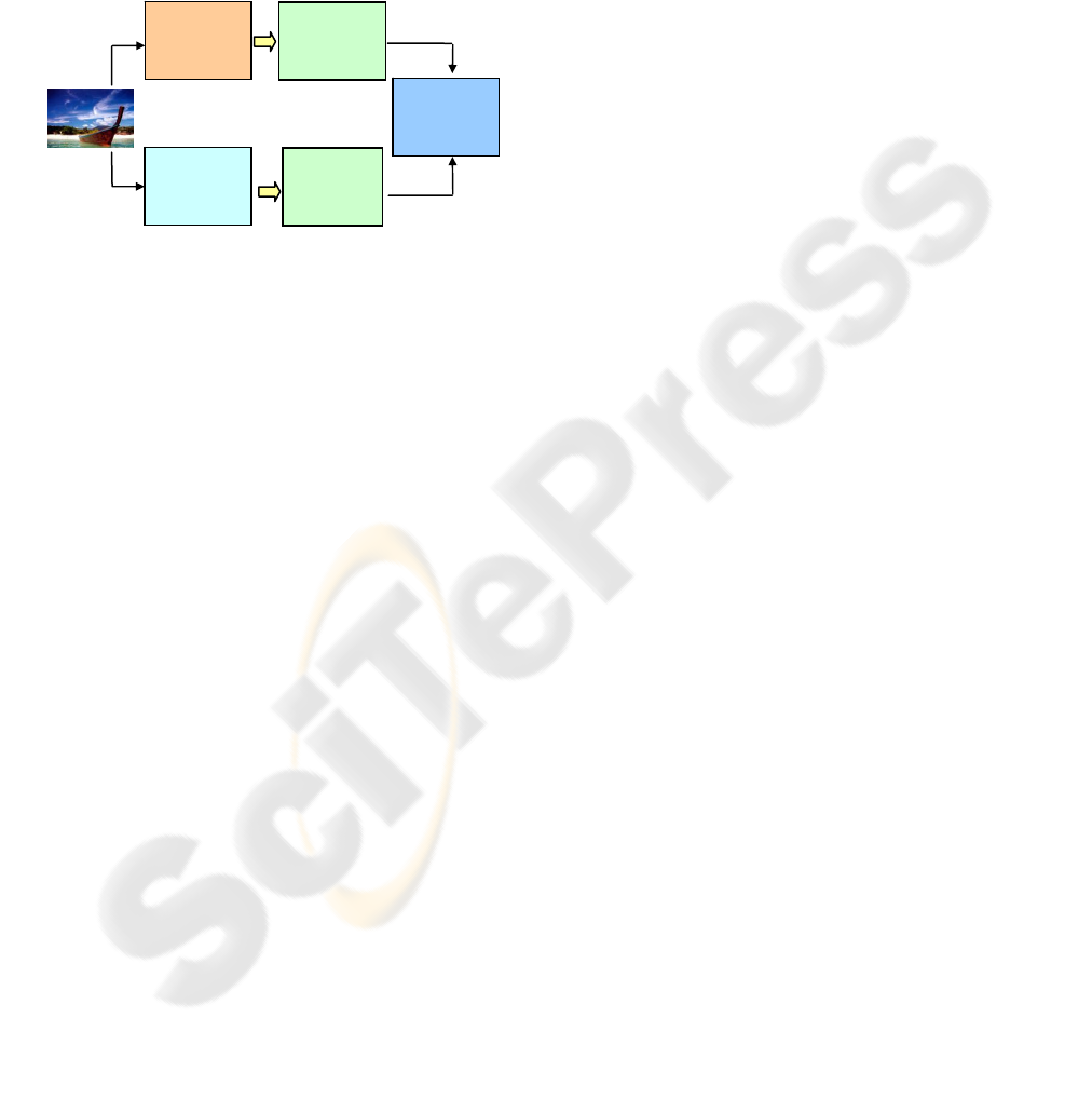
4 INFORMATION FUSION IN AIA
The possibility to extract multiple features from
image data set makes possible building different
visual dictionaries and uses them to represent image
content. The integration of the information conveyed
with different visual terms is not straight, due to the
heterogeneous nature of the different domains, and
needs the employment of a strategy.
Figure 3: Information fusion from different feature types.
Below are presented fusion information strategies to
overcome this gap.
For each different visual dictionary, a LDF
classifier is trained using as input the image set
coded according to the relative visual terms. When a
new image is presented to the system each classifier
produces the N dimensional output whose values are
the scores produced by the g-units. The input image
can be therefore represented by P N-dimensional
vectors, where P is the number of available visual
dictionaries and N the number of the labels.
This representation is used as input for the
information fusion techniques. We have considered
three techniques able to merge the g-scores
information and have compared the results achieved
by them. The techniques are:
a) C5 Decision Tree
b) Weighted Sum of g-scores
c) Higher Level Linear Discriminant
Function
C5 Decision Tree
The set of all the g-units values for the entire
training set has been used to build a decision tree
according the ID3 algorithm (Mitchell, 1997). In
particular, the C5.0/See software has been used
(Quinlan, 2006). Each node discriminates the input
values according one attribute of the input (in this
case the score of a specific g-unit) and redirects the
elaboration to one or another branch according to the
score value. The tree is built placing the nodes
accordingly to information theory criteria such as the
“information gain” that is strictly related to
information entropy of the training data. The leaves
allow to associate a label to the input image.
Weighted sum of g-scores
The value of each g-unit, contained in a LDF
classifier, represents the score of each category
according to the particular LDF visual feature.
Considering to have P visual dictionaries, and
therefore P LDFs, the same number of g-scores for
each label is available. These values are summed
together, with a weight, to have a score dealing with
all the visual dictionaries.
In the Equation (13) is shown the generic label
score achieved with all the P different visual
dictionaries. The g* scores are used to select the
output labels with equations analogue to equation (5)
and equation (6). If the weights φ are set to an equal
fixed value each feature gives the same contribution
to the global score.
Higher level Linear Discriminant Function
The scores of the g-units, equal in number to the
number of labels for the number of LDFs for each
input images, are used to train a higher level LDF
classifier that summarizes the lower LDF outputs.
The output of the higher level LDF (HL LDF)
will be the function of the units trained with this new
training set. The underlying hypothesis is that the
representation achieved in the space of the scores
allows a hyperplane to better discriminate the single
categories.
In the case we consider to characterize images
with two features, for example one for color and the
other for texture, each image is therefore represented
as 2*N values, where N is the number of labels. The
output will be function of the g-units according to
functions analogue to equation (5) and equation (6).
5 EXPERIMENTAL RESULTS
The data set used for the experiments is composed
by 5000 images in JPEG format divided in 50
classes. The training set has been formed with 4500
images while the remaining 500 images have been
used for the test set.
Images are partitioned with a grid of blocks
16x16 pixels. The regular partitioning, although less
able to adapt to data, allows characterizing visual
input in a regular way independently by the
),(),(),(
1
,
** i
jj
Pi
i
jjijj
XgXXg ΛΛ=Λ
∑
≤≤
ϕ
(13)
VISAPP 2007 - International Conference on Computer Vision Theory and Applications
64

robustness of the segmentation algorithm. The same
solution has been adopted by Mori et al. (1999) and
Jeon et al. (2004).
The test and training images have been
characterized with color and texture features. The
color information is represented evaluating RGB
histograms of the image blocks. The texture
information is represented associating to each block
its Gabor Filter Energy histograms.
For all the images of the training set the color
and texture features have been computed. The set of
the values through the LBG algorithm have been
used to form the visual dictionary (one for each
feature). The number of visual terms (equal to the
size of the codebook) has been fixed to 128. The
images have been coded considering the statistics, in
all the blocks, in terms of unigrams and bigrams
with vectors composed by 16512 elements. For each
visual dictionary a LDF has been trained setting the
parameter η in equation (9) equal to 5.
The experiments have been done considering a
variable set of classes and in particular with 5, 20
and 50 classes to test the fusion information
techniques when input values spreading is increased.
The g-scores, produced by the trained LDFs (the
first for the color feature and the second for the
texture feature), have been used as input for the
fusion information step.
The C5 decision tree has been created with the
See5/C5.0 software (Quinlan, 2006) with all the
default parameters and setting the pruning parameter
to the 25%. The performance of the information
fusion has been evaluated considering a single label
assigned to the input image in terms of Det Error.
The results for the decision trees are shown in Table
1.
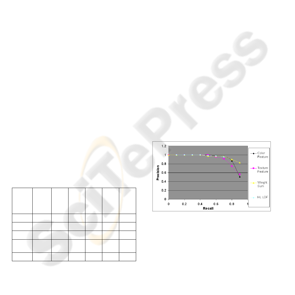
Table 1: Det Error for the training and test error.
Train
Set
Error
N=5
Test
Set
Error
N=5
Train
Set
Error
N=20
Test
Set
Error
N=20
Train
Set
Error
N=50
Test
Set
Error
N=50
Color 0.63 7,67 8.82 31.17 14.72 36.12
Texture 0.63 11.77 10.29 35.14 19.39 42.85
DT (c5) 0.00 7.52 2.26 38.62 9.42 41.94
Weight
ed Sum
0.00 3.80 5.87 31.78 11.70 38.26
HL LDF 0.00 3.80 7.25 33.08 22.70 38.57
Regarding the decision tree, the results in table
show that in the cases the number of classes is 5, the
decision trees perform better that the LDFs trained
with single feature values. When the number of
classes is increased, the performance tends to be an
average of the single feature LDFs performance.
Furthermore a big difference, in terms of Det Error,
is produced between train and test images set. This
difference can be attributed to the limited
generalization capability of the decision tree.
Table 1 shows also that the other fusion
techniques perform better than decision trees and
typically over perform the results achieved by the
single feature LDFs.
The results of these fusion methods, as the
weighted sum of the g-scores and the HL LDF are
compared, in the above figures, through the
precision and recall analysis. The variation of the
threshold in the annotation process (Equation(6))
affects the number of retrieved images. With higher
values of the threshold, fewer labels are retrieved
and so the recall (that is the number of relevant
retrieved images above the number of relevant
images) is low while the precision (the number of
relevant retrieved images above the number of
relevant images) is typically high.
With lower values of the threshold more samples
are retrieved, the recall is increased but the precision
is necessarily diminished. This kind of analysis is
often used in document retrieval but also in image
retrieval field it has proven useful for performance
appraisal (Landgrebe et al., 2006).
The plotting for 5, 20 and 50 classes of precision
versus recall are shown in the Figure 4, Figure 5 and
Figure 6.
Figure 4: Precision versus recall for image data set of 5
Classes.
In Figure 4 is shown the plot of the precision
versus the recall for the described fusion techniques
compared to the performance achieved by the single
features (RGB histograms and Gabor energy
histograms) when the number of classes is set to 5.
The weighted sum of the single scores produces
the best performance among the fusion techniques
and improves the performance of the single feature
annotation too.
INFORMATION FUSION TECHNIQUES FOR AUTOMATIC IMAGE ANNOTATION
65

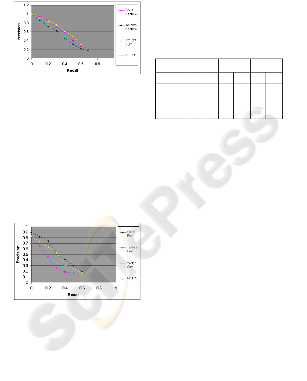
Figure 5: Precision versus recall for image data set of 20
Classes.
When the number of classes is 20 (Figure 5), the
fusion technique using the weighted sum of the g-
scores performs better than the other techniques and
the results of single features are over performed.
The fusion with the LDF in cascade to the single
feature LDF (HL LDF) achieves results that are
intermediate between the performances based on
single features. The results are, for the same value of
recall, less precise than in the 5 classes experiments.
This behaviour can be attributed to the fact that
the scores given by the single features LDF produce
a less evident discrimination among class.
Notwithstanding, the weighted sum of the scored
still allows a good discrimination.
Finally, the performance for 50 classes is shown
in Figure 6. In this case both the fusion techniques of
weighted sum and LDF achieve results that are the
between the performance of the single feature LDFs.
Figure 6: Precision vs Recall for the fusion techniques
applied to the Automatic Annotation of 50 Classes.
The annotation results, achieved with LDF
trained with color features, for the most of values of
the recall parameter, produce better results than the
other fusion techniques. In this case, due to the
increased scattering of the feature values, the
representation in the feature space does not allow a
clear interclass separation and fusion techniques
cannot exploit the multiple features representation.
In Table 2 are shown the False Positive Rate and
False Negative Rate achieved for the input set
formed by 5, 20 and 50 classes when five labels are
associated to each image.
Table 2: False Positive and False Negative rates for the
fusion techniques when 5 labels are assigned to the input
images.
5 Classes 20 Classes 50 Classes
FP FN FP FN FP FN
Color 0.00 0.00 1.31 22.86 0.65 31.80
Texture 0.00 0.00 1.87 27.38 1.00 49.04
Weight. Sum 0.00 0.00 1.38 21.79 0.75 36.60
HL LDF 0.00 0.00 1.16 22.94 0.82 40.40
Due to the definition for False Positive (number
of wrongly annotated images above the number of
negative samples) and False Negative error rates
(number of wrongly not annotated images above the
number of positive samples), their value in the
multi-class case can be very different as the table
shows. The reason is mainly due to different values
of the value of negative samples (denominator of
False Positive Rate) and the number of positive
samples (denominator of False Negative Rate). For
example, for 50 classes the number of positive
sample, in the test set, for each label is 10 set while
the number of negative samples is 490. The error
rates are accordingly affected.
The results in Table 2 confirm the results of the
precision-recall analysis also when multiple labels
are associated to the images. The weighted sum of
the g-scores achieves the best results among the
fusion techniques, while the number of input classes
is 20 or less it over performs the results achieved by
the single feature LDF. When the number of classes
is increased the color feature LDF achieves better
results while the fusion techniques produce results
between the results of the single feature LDFs.
The values of the errors show that the annotation
with this technique can be reliably performed when
the labels are well represented by the LDF scores
and it typically happens when the spreading of the
visual terms in the training set is limited. When the
inter-class value spreading is excessive (increasing
number of classes) other models should be applied
for the single feature representation.
In the below table are compared precision and
recall of the fusion technique adopting the weighted
sum of the g-score for the classification of fifty
classes with the published results of the state of art
VISAPP 2007 - International Conference on Computer Vision Theory and Applications
66

annotation techniques. The proposed technique show
a good improvement although must be said that a
straight comparison is impossible due to the
different adopted features and the number of classes.
Table 3: Comparision of proposed technique with state of
art annotation techniques.
TM
CMR
M
ME MBRM
Propo
sed
Tech.
Prec 0.06 0.10 0.09 0.24 0.36
Recall 0.04 0.09 0.12 0.25 0.36
6 CONCLUSION AND FUTURE
WORKS
Image annotation needs to exploit information from
different orthogonal features to capture the visual
elements carrying a symbolic meaning matched with
the text labels.
The shown techniques use information from
different features and merge together visual
information represented in term of scores related to
different labels. Different information fusion
techniques have been compared showing that, for
this application, the weighted sum of g-scores
produces better results than other fusion techniques.
The information fusion produced putting a HL
LDF to summarize the results of the first stage
LDFs, allows an improvement in performance when
the characterization of input images, through g-units
scores, is adherent to their content. Decision trees
have a reduced utility in this case mainly due to the
reduced generalization capability.
Further investigations will be focused on the
training of the images in terms of more specific
classes or sub-classes that despite a reduced number
of samples for each category are more specific as
content. The application of more complex models
instead of LDF can also allow capturing the positive
and negative classes in a more flexible way and
allow a better performance for fusion algorithms.
ACKNOLEDGEMENTS
Authors would like to thank Kobus Barnard and
Shen Gao for their help with the images data set and
Rulequest company for the evaluation version of the
See5/C5.0 software for decision trees building.
REFERENCES
Barnard K., Duygulu P., Forsyth D., de Freitas N., Blei D.,
Jordan. M., 2003, “Matching words and pictures”,
Journal of Machine Learning Research, Vol.3, pp
1107-1135.
Bellegarda J.-R., 2000, “Exploiting latent semantic
information in statistical language modelling”, Proc.
of the IEEE, Vol. 88, No. 8, pp 1279-1296.
Blei D., Jordan M.-I., 2003, “Modeling annotated data”,
ACM SIGIR.
Carbonetto P., de Freitas N., Barnard K., 2004, “A
statistical model for general contextual object
recognition”, Proc. of ECCV.
Duygulu P., de Freitas N., Barnard K., Forsyth D., 2002,
“Object recognition as machine translation: Learning a
lexicon for a fixed vocabulary”, Proc. of ECCV.
Feng S.-L., Manmatha R., Lavrenko V., 2004, “Multiple
Bernoulli relevance models for image and video
annotation,” , Proc of CVPR’04.
Gao S., Wang D.-H., Lee C.-H., 2006, “Automatic Image
Annotation through Multi-Topic Text Categorization”,
Proc. of ICASSP.
Gao S., Wu W., Lee C.-H., Chua T.-S. , 2004, “A MFoM
learning approach to robust multiclass multi-label text
categorization”, Proc. of ICML.
He X.-M., Zemel R. S., Carreira-Perpiñán M. A., 2004,
“Multiscale conditional random fields for automatic
image annotation”, Proc. of CVPR
Jeon J., Manmatha R., 2004., “Using maximum entropy
for automatic image annotation”, Proc of ICVR.
Jeon J., Manmatha R., 2003, “Automatic image annotation
and retrieval using cross-media relevance models”,
ACM SIGIR.
Landgrebe T.C.W., Paclik P., Duin R.P.W., Bradley A.P.,
2006, "Precision-recall operating characteristic (P-
ROC) curves in imprecise environments", Proc. of the
18th Int. Conf. on Pattern Recognition
Linde Y., Buzo A., Gray R., 1980. “An Algorithm for
Vector Quantizer Design”. IEEE Transaction on
Communications, vol. 28 (1), pp 84–94.
Mitchell T.M., 1997, Machine Learning, McGrawHill
Mori Y, Takahashi H., Oka R., 1999, Image-to-word
transformation based on dividing and vector
quantizing images with words, In Proc of MISRM'99
Quinlan J.R., 2006, Data Mining Tools See5 and C5.0,
from Rule Quest web site: www.rulequest.com/ see5-
info.html
Salton G., 1971, The SMART Retrieval System, Prentice-
Hall, Englewood Cliffs, NJ
Sebastiani F., 2002, “Machine Learning in Automated
Text Categorization”, ACM Computer Surveys, Vol.
34, No. 1, pp 1-47.
Wang D.-H, Gao S., Tian Q., Sung W.-K, 2005,
“Discriminative fusion approach for automatic image
annotation”, Proc. of IEEE 7
th
Workshop on
Multimedia Signal Processing
INFORMATION FUSION TECHNIQUES FOR AUTOMATIC IMAGE ANNOTATION
67