IMPROVED ROBUSTNESS OF MULTIVARIABLE MODEL
PREDICTIVE CONTROL UNDER MODEL UNCERTAINTIES
Cristina Stoica, Pedro Rodríguez-Ayerbe and Didier Dumur
Department of Automatic Control, Supélec, 3 rue Joliot Curie, F91192 Gif-sur-Yvette, France
Keywords: Model Predictive Control (MPC), Multivariable Systems, Linear Matrix Inequalities, Robust Control.
Abstract: This paper presents a state-space methodology for enhancing the robustness of multivariable MPC
controlled systems through the convex optimization of a multivariable Youla parameter. The procedure
starts with the design of an initial stabilizing Model Predictive Controller in the state-space representation,
which is then robustified under modeling errors considered as unstructured uncertainties. The resulting
robustified MIMO control law is finally applied to the model of a stirred tank reactor to reduce the impact of
measurement noise and modelling errors on the system.
1 INTRODUCTION
Model predictive control strategies are widely used
in industrial applications, resulting in improved
performance, with a practical implementation of the
controller which remains simple. However, starting
with a controller design based on a ‘nominal’ model
of the system, the question of its robustness towards
model uncertainties or disturbances acting on the
system always occurs in an industrial environment.
Some methods in the literature deal with
robustness maximisation, but in the transfer function
formalism (Kouvaritakis et al., 1992), (Yoon and
Clarke, 1995), (Dumur and Boucher, 1998), and
mainly applied to SISO systems, which makes the
generalization to multivariable systems much more
complicated.
The purpose of this paper is to present a
methodology enhancing the robustness of an initial
MIMO predictive controller towards model
uncertainties. The state-space design allows the
robustification process to be handled in a convenient
way. A two-step procedure is followed. An initial
MIMO MPC controller is first designed, its robust-
ness is then enhanced via the Youla parametrization,
without significantly increasing the complexity of
the final control law. The Youla parametrization
allows formulating frequency constraints as convex
optimization, the entire problem being solved with
LMI (Linear Matrix Inequality) techniques.
The paper is organized as follows. Section 2
reminds the main steps leading to the MPC
controller in the state-space representation. Section 3
gives the background material required to formulate
the robustification strategy, from the Youla
parametrization to the robustness criteria under
unstructured uncertainties. The elaboration of the
robustified controller in state-space representation
for this type of uncertainties is further proposed in
Section 4. Section 5 provides the application of this
control strategy to a stirred tank reactor. Section 6
presents some conclusions and further perspectives.
2 MIMO MPC IN STATE-SPACE
FORMULATION
This section focuses on the design of an initial
MIMO MPC law. Compared to approaches proposed
in the literature based on transfer function
formalism, the state-space representation framework
chosen here (Camacho and Bordons, 2004) leads to
a simplified formulation and reduced computation
efforts for MIMO systems. Consider the following
discrete time MIMO LTI system:
⎩
⎨
⎧
=
+=+
)()(
)()()1(
kk
kkk
xCy
uBxAx
(1)
where
nn×
∈
R
A ,
mn×
∈ RB ,
np×
∈RC are the
system state-space matrices,
1×
∈
n
R
x describes the
MIMO system states,
1×
∈
m
Ru
is the input vector
and
1×
∈
p
Ry is the output vector.
Next step is to add an integral action to this
state-space representation which will guarantee
cancellation of steady-state errors:
)()1()( kkk uuu Δ
+
−
=
(2)
283
Stoica C., Rodríguez-Ayerbe P. and Dumur D. (2007).
IMPROVED ROBUSTNESS OF MULTIVARIABLE MODEL PREDICTIVE CONTROL UNDER MODEL UNCERTAINTIES.
In Proceedings of the Fourth International Conference on Informatics in Control, Automation and Robotics, pages 283-288
DOI: 10.5220/0001651002830288
Copyright
c
 SciTePress

This results in an increase of the system states as:
⎩
⎨
⎧
=
Δ+=+
)()(
)()()1(
kk
kkk
ee
eeee
xCy
uBxAx
(3)
where the extended state-space representation
[]
T
TT
e
kkk )1()()( −= uxx is characterized by:
⎥
⎦
⎤
⎢
⎣
⎡
=
mnm
e
I0
BA
A
,
,
⎥
⎦
⎤
⎢
⎣
⎡
=
m
e
I
B
B
,
[]
mpe ,
0CC =
.
The control signal is derived by minimizing the
following quadratic objective function:
∑
∑
−
=
=
+Δ+
++−+=
1
0
2
)(
~
2
)(
~
)(
)()(
ˆ
2
1
u
J
J
N
i
i
N
Ni
i
ik
ikikJ
R
Q
u
wy
(4)
where the future control increments
)( ik
+
Δu
are
supposed to be zero for
u
Ni ≥ . The signal w
represents the setpoint. It is assumed in further
developments that the same output prediction
horizons (
1
N ,
2
N ) and the same control horizon
u
N is applied for all input/output transfer functions.
J
Q
~
and
J
R
~
are weighting matrices. The predicted
output vector has the following form:
∑
−
=
−−
++=+
1
0
1
)()(
ˆ
)(
ˆ
i
j
jii
jkkik BuACxACy
(5)
where the input vector can be written as:
∑
=
+Δ+−=+
j
l
lkkjk
0
)()1()( uuu
(6)
The state estimate is derived from the observer:
])(
ˆ
)([)()(
ˆ
)1(
ˆ
kkkkk
eeeeee
xCyKuBxAx −+Δ+=+
(7)
The multivariable observer gain
K
is designed
through a classical method of eigenvectors,
arbitrarily placing the eigenvalues of
ee
CKA − in
a stable region, as detailed in (Magni
, 2002). The
observer gain
K
is obtained from the extended
state-space description and will be used for further
mathematical calculation in the robustification
procedure. However this design aspect is not crucial
since the convex robustification method should lead
to an optimal set of these eigenvalues. Moreover the
input/output transfer function is not influenced by
the eigenvalues placement used to find
K
(Boyd
and Barratt, 1991).
The objective function can be rewritten in the
matrix formalism (Maciejowski, 2001):
22
)()()(
JJ
kkkJ
RQ
UWY Δ+−=
(8)
where ))(
~
,),(
~
(
21
NNdiag
JJJ
QQQ "= ,
))1(
~
,),0(
~
( −=
uJJJ
Ndiag RRR " ,
[
]
T
TT
NkNkk )(
ˆ
)(
ˆ
)(
21
++= yyY " ,
[
]
T
TT
NkNkk )()()(
21
++= wwW " ,
[
]
T
u
TT
Nkkk )1()()( −+ΔΔ=Δ uuU " .
Using these notations, the output vector )(kY can be
written in the following matrix form, with the
definition of the vector
)(kΘ as a tracking error:
)()1()(
ˆ
)( kkkk UΦuΦxΨY Δ+
−
+
=
Δ
(9)
)1()(
ˆ
)()( −−
−
=
kkkk uΦxΨWΘ
(10)
with
[
]
T
T
N
T
N
)()(
21
CACAΨ "= ,
[
]
T
T
N
T
N 11
21
−−
= ΣΣΦ "
,
∑
=
−
=
i
j
ji
i
0
BACΣ ,
T
i
T
i
)(ΣΣ = ,
⎥
⎥
⎥
⎦
⎤
⎢
⎢
⎢
⎣
⎡
=
−−−−−
−
Δ
u
NNNNNNN
N
212122
1
11
01
00
ΣΣΣΣ
ΣΣ
Φ
""
#%##"#
""
.
The objective function is now given by:
22
)()()(
JJ
kkkJ
RQ
UΘUΦ Δ+−Δ=
Δ
(11)
which analytical minimization provides:
)()()(
T1T
kk
JJJ
ΘQΦΦQΦRU
Δ
−
ΔΔ
+=Δ
(12)
Applying the receding horizon principle, only the
first component of each future control sequence is
applied to the system, meaning that the first m lines
of
)(kU
Δ
are used:
)()( kk Θμu
=
Δ
(13)
with
[
]
JJJNmmm
u
QΦΦQΦR0Iμ
T1T
)1(,
)(
Δ
−
ΔΔ−
+= .
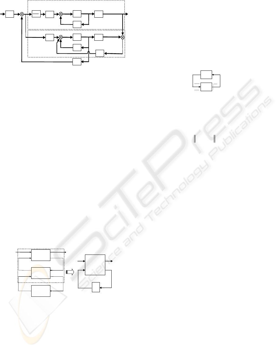
The system model, the observer and the
predictive control can be represented in the state-
space formulation according to Figure 1. The control
signal depends on the control gain
[]
21
LLL = and
the setpoint filter
w
F :
)(
ˆ
)()( kkk
ew
xLwFu
−
=
Δ
(14)
with μΨL
=
1
, μΦL
=
2
,
),,(
,1, pwww
diag FFF "=
related to the structure of
μ
and )(kw .
ICINCO 2007 - International Conference on Informatics in Control, Automation and Robotics
284

q
-1
q-1
q
-
+
+
+
+
+
+
+
-
x
e
(k) x
e
(k+1)
L
K
q
-1
A
C
e
A
e
B
e
F
w
y
(k)
x(k) x(k+1)
Δu(k) u(k)
w(k)
MIMO system
observer
B C
y
’(k)
^
^
Figure 1: Block diagram of MIMO MPC.
3 ROBUSTNESS USING THE
YOULA PARAMETER
This section overviews a technique that improves the
robustness of the previous multivariable MPC law in
terms of the Youla parameter, also named
Q
parameter. Any stabilizing controller (Boyd and
Barratt, 1991), (Maciejowski, 1989) can be
represented by a state-space feedback controller
coupled with an observer and a Youla parameter.
This part focuses on the main steps leading to the
multivariable
Q parameter (here with p inputs and
m outputs) that robustifies the MPC law described
in Section 2.
3.1 Stabilizing Control Law
The whole class of stabilizing control law can be
obtained from an initial stabilizing controller via the
Youla parametrization. The first step considers
additional inputs
u
′
and outputs y
′
with a zero
transfer between them ( 0
22
=T in Figure 2).
z
w
Q
p
aramete
r
Initial
controlle
r
MIMO
System
y
u ’
y
’
u
y
’
Q
u ’
⎟
⎟
⎠
⎞
⎜
⎜
⎝
⎛
2221
1211
TT
TT
z
w
Figure 2: Class of all stabilizing multivariable controllers.
The Youla parameter is then added between y
′
and
u
′
without restricting closed-loop stability. In this
case, the transfer from
u
to
y
remains unchanged.
As a result, the closed-loop function between w and
z is linearly parametrized by the Q parameter, allo-
wing convex specification (Boyd and Barratt, 1991):
zwzwzw
TQTTT
zw 211211
+=
(15)
where
211211
,, TTT depends on the input vector
w and output vector z considered.
3.2 Robustness Under Frequency
Constraints
Practical applications always deal with neglected
dynamics and potential disturbances, so that
robustness under unstructured uncertainties must be
addressed as shown in Figure 3.
u
Δ
z
w
zw
T
Figure 3: Unstructured uncertainty.
According to the small gain theorem
(Maciejowski, 1989), robustness under unstructured
uncertainties
u
Δ
is maximized as:
∞
ℜ∈
∞
T
H
WT
zw
Q
min
(16)
where the weighting term
T
W reflects the frequency
range where model uncertainties are more important.
For multivariable systems, the
∞
H norm can be
calculated as the maximum of the higher singular
values. The following theorem formulates the
previous
∞
H norm minimization.
Theorem (Clement and Duc, 2000) and (Boyd et al.,
1994): A discrete time system given by the state-
space representation
),,,(
clclclcl
DCBA
is stable
and admits a
∞
H norm lower than
γ
if and only if:
0/0
TT
T
1
T
1
1
T
11
<
⎥
⎥
⎥
⎥
⎦
⎤
⎢
⎢
⎢
⎢
⎣
⎡
−
−
−
−
>=∃
−
IDC0
DI0B
C0XA
0BAX
XX
γ
γ
clcl
clcl
clcl
clcl
(17)
This expression can be transformed into a LMI,
which variables are
1
X ,
γ
and the Q parameter
included in the closed-loop matrices, as shown in
(Clement and Duc, 2000). As a result, the
optimization problem is formulated as the
minimization of
γ
under this LMI constraint.
4 ROBUSTIFIED MIMO MPC
The previous robustification strategy based on the
Youla parameter is now applied to an initial MIMO
state-space MPC calculated as shown in Section 2.
The robustness maximization under additive
unstructured uncertainties is also equivalent to the
minimization of the influence of a measurement
noise
b on the control signal
u
(Figure 4); the
IMPROVED ROBUSTNESS OF MULTIVARIABLE MODEL PREDICTIVE CONTROL UNDER MODEL
UNCERTAINTIES
285

transfer (15) between
w
and z corresponds to the
transfer from
b to u . The
∞
H norm of this transfer
will be further minimized using LMI tools.
+
∆
u
+
z
(
k
)
W
u
Q
-
+
b(k)
+
+
+
+
+
+
+
-
q- 1
q
x
e
(k) x
e
(k+1)
L
K
q
-1
q
-1
A
C
e
A
e
B
e
F
w
y
(k)
x(k) x(k+1)
Δu(k) u(k)
w(k)
d(k)
MIMO system
observer
B C
y
’(k)
^
^
u’(
k
)
+
-
Figure 4: Stabilizing MIMO MPC via Q parametrization.
4.1 Stabilizing Control Law
Consider the MIMO linear discrete time system in
the state-space representation, including an integral
action (3). After adding an auxiliary input vector
u
′
and output vector
y
′
(Figure 4), the multivariable
control signal is computed as described in Section 2:
)()(
ˆ
)()( kkkk
ew
uxLwFu
′
−−=Δ
(18)
with the following observer:
)]()(
ˆ
)([
)()(
ˆ
)1(
ˆ
kkk
kkk
ee
eeee
bxCyK
uBxAx
+−+
+Δ+=+
(19)
To calculate the closed-loop transfer function, the
initial state is increased, adding the prediction error:
)(
ˆ
)()( kkk
ee
xxε
−
=
(20)
Considering only the terms related to )(kb as they
are part of the minimization process, the following
state-space system is derived:
⎥
⎦
⎤
⎢
⎣
⎡
′
⎥
⎦
⎤
⎢
⎣
⎡
−
−
+
⎥
⎦
⎤
⎢
⎣
⎡
⎥
⎦
⎤
⎢
⎣
⎡
=
⎥
⎦
⎤
⎢
⎣
⎡
+
+
)(
)(
)(
)(
)1(
)1(
2
31
k
k
k
k
k
k
eee
u
b
0K
B0
ε
x
A0
AA
ε
x
(21)
[] []
⎥
⎦
⎤
⎢
⎣
⎡
′
+
⎥
⎦
⎤
⎢
⎣
⎡
=
′
)(
)(
)(
)(
)(
k
k
k
k
k
e
e
u
b
0I
ε
x
C0y
(22)
with LBAA
ee
−=
1
,
ee
KCAA −
=
2
, LBA
e
=
3
.
According to the theory given in Section 3.1, the
Youla parameter can be added to robustify the initial
controller, since the transfer between
)(ky
′
and
)(ku
′
is zero (without measurement noise, the
multivariable output
y
′
depends only on )(kε ,
which is independent from
)(k
e
x and )(ku
′
).
4.2 Robustness Under Frequency
Constraints
Next step is the definition of the weighting
u
W as a
diagonal high-pass filter in state-space formulation:
⎩
⎨
⎧
+=
+=+
)()()(
)()()1(
kkk
kkk
www
wwww
uDxCz
uBxAx
(23)
Including the
u
W weighting, a new extended
state-space description can be emphasized:
⎥
⎦
⎤
⎢
⎣
⎡
′
⎥
⎦
⎤
⎢
⎣
⎡
−
−
+
⎥
⎦
⎤
⎢
⎣
⎡
⎥
⎦
⎤
⎢
⎣
⎡
=
⎥
⎦
⎤
⎢
⎣
⎡
+
+
′
)(
)(
)(
)(
)1(
)1(
1
2
31
1
k
k
k
k
k
k
u
u
b
0K
B0
ε
x
A0
AA
ε
x
(24)
⎥
⎦
⎤
⎢
⎣
⎡
′
⎥
⎦
⎤
⎢
⎣
⎡
−
+
⎥
⎦
⎤
⎢
⎣
⎡
⎥
⎦
⎤
⎢
⎣
⎡
=
⎥
⎦
⎤
⎢
⎣
⎡
′
)(
)(
)(
)(
)(
)(
1
21
k
k
k
k
k
k
w
e
u
b
0I
D0
ε
x
C0
CC
y
z
(25)
with
[
]
T
T
w
TT
kkkk )()1()()(
1
xuxx −= ,
[]
T
T
w
T
u
BIBB =
′
⎥
⎥
⎦
⎤
⎢
⎢
⎣
⎡
−−
−−
−−
=
www
ALIBLB
0LIL
0BLBBLA
A
)(
21
21
21
1
,
⎥
⎥
⎦
⎤
⎢
⎢
⎣
⎡
=
LB
L
BL
A
w
3
,
[
]
www
CLIDLDC )(
211
−−= , LDC
w
=
2
.
As described in Section 3.2, a multivariable Youla
parameter
∞
ℜ
∈
HQ is added for robustification
purposes leading to a convex optimization problem.
Since this problem leads to a
Q parameter which
varies in the infinite-dimensional space
∞
ℜH , a
sub-optimal solution considers for each input/output
pairs
),( ji a finite-dimensional subspace generated
by an orthonormal base of discrete stable transfer
functions such as a polynomial or FIR filter:
∑
=
−
=
Q
n
l
l
ij
l
ij
qqQ
0
(26)
In the state-space formalism, this MIMO Youla
parameter can be obtained using a fixed pair
),(
ppn
Q
pnpn
Q
QQQ
××
∈∈ RBRA and designing
only the variable pair
),(
pm
Q
pnm
Q
Q
×
×
∈∈ RDRC :
⎩
⎨
⎧
′
+=
′
′
+=+
)()()(
)()()1(
kkk
kkk
QQQ
QQQQ
yDxCu
yBxAx
(27)
with
⎥
⎥
⎦
⎤
⎢
⎢
⎣
⎡
=
−−
−
1,11
1,1
0
QQ
Q
nn
n
Q
0I
0
a
,
⎥
⎦
⎤
⎢
⎣
⎡
=
− 1,1
1
Q
n
Q
0
b
,
⎥
⎥
⎥
⎦
⎤
⎢
⎢
⎢
⎣
⎡
=
ij
n
ij
ij
Q
Q
q
q
#
1
c
⎥
⎥
⎥
⎦
⎤
⎢
⎢
⎢
⎣
⎡
=
mp
Q
m
Q
p
Q
Q
Q
cc
cc
C
"
#%#
"
1
1
11
,
⎥
⎥
⎥
⎦
⎤
⎢
⎢
⎢
⎣
⎡
=
mp
m
p
Q
qq
qq
0
1
0
1
0
11
0
"
#%#
"
D
,
),,(
QQQ
diag aaA "
=
, ),,(
QQQ
diag bbB "= .
Adding this Youla parameter leads to the following
closed-loop state-space description:
⎩
⎨
⎧
+=
+=+
)()()(
)()()1(
kkk
kkk
clclcl
clclclcl
bDxCz
bBxAx
(28)
with
[
]
T
T
Q
TT
cl
xεxx
1
=
,
ICINCO 2007 - International Conference on Informatics in Control, Automation and Robotics
286

[]
QweQwcl
CDCDDCCC −−=
21
,
Qwcl
DDD
−
=
,
⎥
⎥
⎥
⎦
⎤
⎢
⎢
⎢
⎣
⎡
−−
=
′′
QeQ
QueQu
cl
ACB0
0A0
CBCDBAA
A
2
31
,
⎥
⎥
⎥
⎦
⎤
⎢
⎢
⎢
⎣
⎡
−
−
=
′
Q
Qu
cl
B
K
DB
B
.
This state-space representation is the crucial point of
the robustification method. With the result of the
theorem in Section 3, the first step to transform (17)
into a LMI consists in multiplying it to the right and
to the left with positive definite matrices
),,,(diag
1
IIIXΠ = and
T
Π as in (Clement and
Duc, 2000). This leads to the following inequality:
0
T
1
T
T
11
T
111
<
⎥
⎥
⎥
⎥
⎦
⎤
⎢
⎢
⎢
⎢
⎣
⎡
−
−
−
−
IDC0
DI0XB
C0XXA
0BXAXX
γ
γ
clcl
clcl
clcl
clcl
(29)
which is not yet a LMI because terms such as
cl
AX
1
and
cl
BX
1
are not linear in
1
X
,
Q
C and
Q
D . To
overcome this problem, the following bijective
substitution is introduced (Clement and Duc, 2000):
⎪
⎪
⎩
⎪
⎪
⎨
⎧
⎥
⎥
⎥
⎦
⎤
⎢
⎢
⎢
⎣
⎡
=
⎥
⎦
⎤
⎢
⎣
⎡
⎥
⎦
⎤
⎢
⎣
⎡
=
→
××
221212
121111
12111
1
T
1
11
1
T
1
11
1
TTS
TTS
SSR
TS
SR
YZ
ZW
X
RR
TT
T
nnnn
6
(30)
with
1
11
−
= WR ,
1
1
11
ZWS
−
−= ,
1
1
1
T
111
ZWZYT
−
−= .
Next step to the LMI is to multiply (29) on the right
with
⎟
⎟
⎠
⎞
⎜
⎜
⎝
⎛
⎥
⎦
⎤
⎢
⎣
⎡
⎥
⎦
⎤
⎢
⎣
⎡
= II
IS
0R
IS
0R
Γ ,,,diag
T
1
1
T
1
1
and on the left
with
T
Γ . After technical manipulations, the
following LMI is obtained:
0
*******
******
*****
****
***
**
*
13
1222
111211
101
96322
8521211
741111
<
⎥
⎥
⎥
⎥
⎥
⎥
⎥
⎥
⎥
⎦
⎤
⎢
⎢
⎢
⎢
⎢
⎢
⎢
⎢
⎢
⎣
⎡
−
−
−
−−
−
−
−−
−
I
I
0T
0TT
000R
00T
00TT
0RA00R
γ
γ
t
t
t
t
ttt
ttt
ttt
(31)
where
eQueQ
t CDBACBSASSA
′
−+−−=
3122111111
,
eQ
t CBTAT
122112
+=
,
eQ
t CBTAT
222
T
123
+=
,
QuQ
t CBASSA
′
−−=
121214
,
Q
t AT
125
=
,
Q
t AT
226
=
,
QQu
t BSKSDB
12117
−+−=
′
,
Q
t BTKT
12118
+−=
,
Q
t BTKT
22
T
219
+−=
,
T
1101
CR=t ,
TT
31 wQ
t DD−= ,
TT
2
T
1
T
1111 w
T
Q
T
e
t DDCCCS −+=
,
TTT
1
T
2121 wQ
t DCCS −=
.
The whole problem results in the minimization
of
γ
subject to the LMI constraint (31):
γ
LMI
min
(32)
5 APPLICATION TO A STIRRED
TANK REACTOR
The previous robustification methodology is applied
now to the simplified MIMO model of a stirred tank
reactor presented in the transfer function formalism
in (Camacho and Bordons, 2004):
⎥
⎦
⎤
⎢
⎣
⎡
⎥
⎦
⎤
⎢
⎣
⎡
++
++
=
⎥
⎦
⎤
⎢
⎣
⎡
)(
)(
)4.01/(2)5.01/(1
)3.01/(5)7.01/(1
)(
)(
2
1
2
1
sU
sU
ss
ss
sY
sY
(33)
where
1
Y and
2
Y are the effluent concentration and
the reactor temperature,
1
U and
2
U are the feed
flow rate and the coolant flow, respectively.
Starting from the state-space representation of
this 2 inputs/ 2 outputs model discretized for a
sampling time
03.0=
e
T min, an integral action is
added leading to an extended state-space model. For
simplicity reasons of multivariable MPC, the same
prediction horizons
1
1
=
N ,
3
2
=N
and 2=
u
N
were used for all outputs and control signals, and the
same weights as in (Camacho and Bordons, 2004)
u
NJ
R I05.0
~
=
and
1
12
~
+−
=
NNJ
Q I
.
0 0.5 11.5 2 2.5 3 3.5 4 4.5
0
0.1
0.2
0.3
0.4
0.5
Time
(
minute
)
1
y
2
y
Setpoint
Before robustification
After robustificatio
n
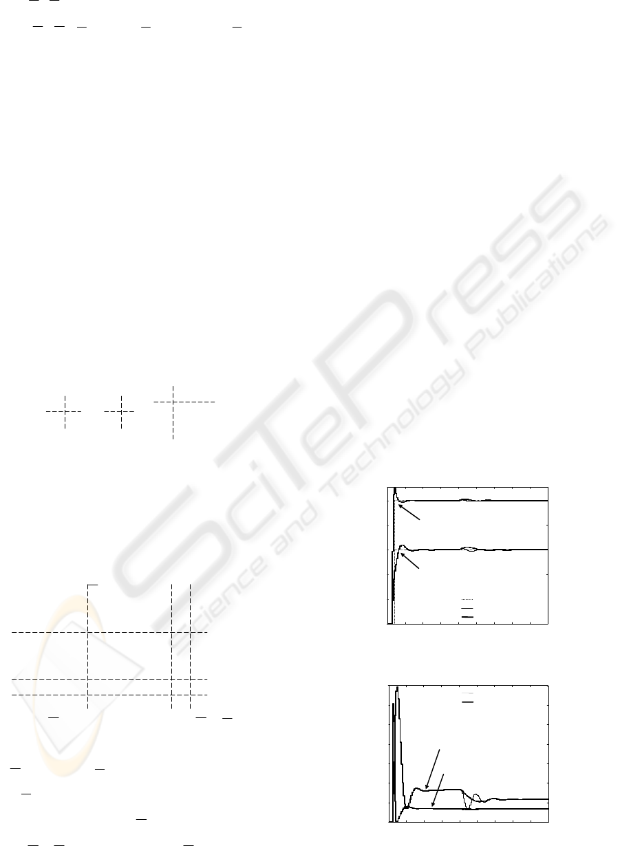
Time Responses
Figure 5:
1
y and
2
y before and after robustification.
0 0.5 11.52 2.5 3 3.5 4
4.5
0
0.1
0.2
0.3
0.4
0.5
0.6
0.7
Time
(
minute
)
1
u
2
u
Before robustification
After robustification
Control Signals
Figure 6:
1
u and
2
u before and after robustification.
IMPROVED ROBUSTNESS OF MULTIVARIABLE MODEL PREDICTIVE CONTROL UNDER MODEL
UNCERTAINTIES
287

Figures 5 shows the time responses obtained for
a step reference of 0.5 for
1
y , and 0.3 for
2
y , and
the disturbance rejection for a step disturbance of
0.05 applied to
1
u at 2=t min. Figure 6 shows the
control signals
1
u and
2
u .
For robustness under additive uncertainties at
high frequency, a high-pass filter is used for each
control signal, as described in Section 4.2 which
transfer form is
3.0/)7.01(
1
2
−
−= qIW
u
. Using
the optimization procedure based on LMIs gives a
multivariable Youla parameter as a
22 × matrix of
polynomials of order
20
=
Q
n .
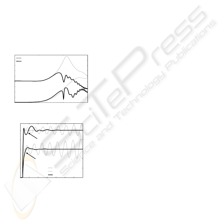
Figure 7 shows the singular values analysis of
transfer from
b to control signals u (from
Figure 4). The greatest value of maximal singular
values represents the
∞
H norm. We can remark that
this
∞
H norm has been reduced. In this way the
stability robustness is improved with respect to high-
frequency additive unstructured uncertainties.
10
-1
10
0
10
1
10
2
-15
-10
-5
0
5
10
15
20
25
30
Frequency (rad/min)
Before robustification
After robustification
Singular Values (dB)
Figure 7: Singular values before and after robustification.
0
0
0.5
1
1.5
2
2.5 3
3.5
0.1
0.2
0.3
0.4
0.5
Time
(
minute
)
1
y
2
y
Setpoint
Before robustification
After robustification
Time Responses
Figure 8:
1
y and
2
y before and after robustification.
Figures 5 and 6 show that after robustification
the input/output behaviour is unchanged, but the
disturbance is rejected more slowly by the
robustified controller. In fact, the robustified
controller has a slower disturbance rejection, but a
higher robust stability. To support this, a high
frequency neglected dynamics of the actuator
1
u has
been considered. Thus the transfer between
11
/ uy
corresponds to
)07.01)(7.01/(1 ss ++ . Figure 8
illustrates that the initial controller behaviour is
destabilized by this uncertainty, but the robustified
controller remains stable; it also shows the influence
of the considered unstructured uncertainty to
2
y .
6 CONCLUSIONS
This paper has presented a new MIMO complete
methodology which enables robustifing an initial
multivariable MPC controller in state-space
formalism using the Youla parameter framework. In
order to improve robustness towards unstructured
uncertainties, a
∞
H convex optimization problem
was solved using the LMIs techniques. The major
advantage of the developed structure is the state-
space formulation of this MPC robustification
problem for MIMO systems with a reduced
computational effort compared to the transfer
function formalism. This method can also be applied
to non square systems, which otherwise are more
difficult to control. This technique enables also the
use of time-domain templates to manage the
compromise between stability robustness and
nominal performance.
REFERENCES
Boyd, S., Barratt, C., 1991. Linear controller design.
Limits of performance, Prentice Hall.
Boyd, S., Ghaoui, L.El., Feron, E., Balakrishnan, V., 1994.
Linear matrix inequalities in system and control
theory, SIAM Publications, Philadelphia.
Camacho, E.F., Bordons, C., 2004. Model predictive
control, Springer-Verlag. London, 2
nd
edition.
Clement, B., Duc, G., 2000. A multiobjective control via
Youla parameterization and LMI optimization:
application to a flexible arm, IFAC Symposium on
Robust Control and Design, Prague.
Dumur, D., Boucher, P., 1998. A Review introduction to
linear GPC and applications, Journal A, 39(4), pp. 21-
35.
Kouvaritakis, B., Rossiter, J.A., Chang, A.O.T., 1992.
Stable generalized predictive control: an algorithm
with guaranteed stability, IEE Proceedings-D, 139(4),
pp. 349-362.
Maciejowski, J.M., 1989. Multivariable feedback design,
Addison-Wesley Publishing Company, Wokingham,
England.
Maciejowski, J.M., 2001. Predictive control with
constrains, Prentice Hall.
Magni, J.F., 2002. Robust modal control with a toolbox for
use with MATLAB, Springer.
Yoon, T.W., Clarke, D.W. 1995. Observer design in
receding-horizon predictive control, International
Journal of Control, 61(1), pp. 171-191.
ICINCO 2007 - International Conference on Informatics in Control, Automation and Robotics
288