A NEW PROBABILISTIC PATH PLANNER
For Mobile Robots Comparison with the Basic RRT Planner
Sofiane Ahmed Ali, Eric Vasselin and Alain Faure
Groupe de Recherce en Electrotechnique Automatique (GREAH) Le Havre University, France
25 Philippe Lebon Street 76058 Le Havre Cedex
Keywords: Robotics, motion planning, rapidly exploring random trees.
Abstract: the rapidly exploring random trees (RRTs) have generated a highly successful single query planner which
solved difficult problems in many applications of motion planning in recent years. Even though RRT works
well on many problems, they have weaknesses in environments that handle complicated geometries.
Sampling narrow passages in a robot’s free configuration space remains a challenge for RRT planners
indeed; the geometry of a narrow passage affects significantly the exploration property of the RRT when the
sampling domain is not well adapted for the problem. In this paper we characterize the weaknesses of the
RRT planners and propose a general framework to improve their behaviours in difficult environments. We
simulate and test our new planner on mobile robots in many difficult static environments which are
completely known, simulations show significant improvements over existing RRT based planner to reliably
capture the narrow passages areas in the configuration space.
1 INTRODUCTION
Motion planning can be defined as finding path for a
mobile device (such a robot) from a given start to a
given goal placement in workspace without colliding
with obstacles in the workspace. Beside the obvious
application within robotics, motion planning also
pays an important role in animation, virtual
environments, computer games, computer aided
design and maintenance, and computational
chemistry.
Despite the success of the earlier deterministic
motion planning algorithms, path planning for a
robot with many degrees of freedom is difficult.
Several instances of the problem have been proven
to be PSPACE-hard (Reif, 1979) or even
undecidable. In recent years random sampling has
emerged as a powerful approach for motion planning
problems. It breaks the computational complexity in
(Reif, 1979) and shows efficiency and its easy way
to implement in high dimensional configuration
space. Current random-sampling based algorithms
can be divided into two sets of approaches: multiple
query and the single query methods
The primary philosophy behind the multiple
query methods is that substantial pre-computational
time may be taken so that multiple queries for the
same environment can be answered quickly. The
probabilistic roadmap method (PRM) (Svestka,
1997) (Kavraki, 1994) is an example of such
method.
The multiple query methods may take
considerable pre-computation time thus; different
approaches were developed for solving single-query
problems. The rapidly exploring random trees
(RRTs) is a popular motion planning technique
which was primarily designed for single-query
holonomic problems and problems with differential
constraints (LaValle, 1998), The success of this
approach provide their extensions to different
motion planning issues from problems with
complicated geometries (Ferré, 2004), to
manipulation problem and motions of closed
articulated chains in, (Yershova and LaValle, 2007).
Adapted versions of RRT for non holonomic and
kinodynamic motions also exists (Lamiraux and
Ferré, 2004),
Even though RRT works well in many
applications, they have several weaknesses, which
cause them to perform poorly in some cases. Narrow
passages are small region which naturally restrict the
movements of the mobile robots in one or many
directions. Leading to a prohibitively many
402
Ahmed Ali S., Vasselin E. and Faure A. (2007).
A NEW PROBABILISTIC PATH PLANNER - For Mobile Robots Comparison with the Basic RRT Planner.
In Proceedings of the Fourth International Conference on Informatics in Control, Automation and Robotics, pages 402-407
DOI: 10.5220/0001649504020407
Copyright
c
 SciTePress

expensive operations (i.e. collision checks) are being
performed during the execution of the algorithm. It
is unlikely that a basic RRTs algorithm can
overcome this major difficulty entirely.
Recently a new probabilistic approach to find
paths through narrow passages areas was proposed
(Ahmed ali, Vasselin, and Faure, 2006). The
approach is based on the idea of adapting the
sampling domain to the geometry of the workspace.
In this paper, we illustrate the weaknesses of the
RRT planner and we propose a general framework
based on the approach (Ahmed Ali, Vasselin, and
Faure, 2006) to minimize the effects of some of
these weaknesses. The result is a simple new planner
that shows significant improvements over existing
RRT planners, in some cases by several orders of
magnitude. The key idea in (Ahmed Ali, Vasselin,
and Faure, 2006) is what we call the Angular-
Domain a specialized sampling strategy for narrow
passages that takes into account the obstacles in the
configuration space. Although the idea is general
enough and should be applicable to other motion
planning problems (e.g. planning for closed chains,
non holonomic planning), we focus in this work only
on holonomic problems.
The remaining part of the paper is organized as
follows. First, the original RRT planers are
presented with an illustration of the Voronoi biased
exploration strategy. In the end of section 2 we
analyze the performance of the RRT algorithm on
one challenging example for the RRT planners.
Section 3 gives a formal characterization of the
Angular Domain as a new sampling strategy for
narrow passages areas Simulations results in case of
holonomic robots are shown in the end of section 3.
a sort summary concludes the paper.
2 THE RRT FRAMEWORK
2.1 General Approach
The rapidly random exploring trees (RRT) are
incremental search algorithm. They incrementally
construct a tree from the initial state to the goal state
(bidirectional versions exists as well). At each step,
a random sample is chosen and its nearest neighbour
in the search tree computed. A new node
(representing a new configuration in the free
configuration space) is then created by extending the
nearest neighbour toward the random sample. See
Figure 1 for the construction of the tree and Figure 2
for a pseudo code of the algorithm.
Figure 1: Incremental construction of a basic RRT tree.
__________________________________________
Build_RRT(
init
q )
1
);.(.
init
qinit
τ
2 for
1
=
k to N do (until the maximum number of
nodes is reached)
3
();_ ConfigRandomq
rand
←
4
),.(_
τ
randnear
qNeighborNearestq
←
5 if CONNECT
),,,(
newnearrand
qqq
τ
;
6
);.(_.
new
qvertexadd
τ
7
);,.(_.
newnear
qqedgeadd
τ
8 if the goal configuration
goal
q is reached then
Exit
Nk
=
Return
Figure 2: The basic RRT algorithm.
2.2 RRT and Voronoi Bias
This exploration strategy has an interesting property:
it is characterized by Voronoi bias. At each iteration,
the probability that a node is selected is proportional
to the volume of its Voronoi region; hence, the
search is biased toward those nodes with the largest
Voronoi regions (the unexplored regions of the
configuration space
2.3 Bug Trap and Narrow Passages
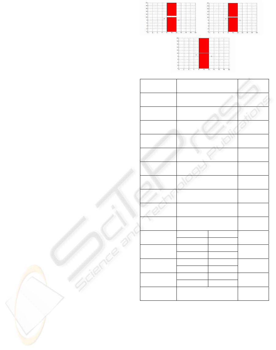
We consider the problems shown in Figure.3 (a). (c).
the task is to move the robot outside the bug trap
1
for the first two figures, and from the left side to the
right side through a narrow passage for the second.
A NEW PROBABILISTIC PATH PLANNER - For Mobile Robots Comparison with the Basic RRT Planner
403

(a) (b) (c)
Figure 3: A bug trap problem and a narrow passage in
high dimension can be very challenging for RRT planners.
The problem become more challenging when the sampling
domain is enlarged (b) and (c).
The tree constructed by the RRT planner in the
bug trap is shown in blue and the Voronoi region
associated with the nodes of the tree are shown in
red Figure.3.a. A frontier node are vertices in the
tree that has their Voronoi region growing together
with the size of the environment, while a boundary
node are those that lie in some proximity to the
obstacles. Note that frontier nodes are suitable for
the RRT planners because they provide a strong bias
toward the unexplored portions of the configuration
space. The problem is that given the geometry of the
narrow passages a frontier node is usually a
boundary node, since that the boundary nodes are
given more Voronoi bias than they can explore;
prohibitively many expensive operations are being
performed during the execution of the RRT. Finally
the tree in the middle of the bug trap or in the
narrow passage does not grow at all leading to a
considerable slow-down in the performance of the
RRT.
Thus, the goal of this paper is to find a way of
reducing the number of expansive iterations in RRT.
The obvious solution to this problem would be to
limit the sampling domain to get more nodes in the
middle of the bug trap and the narrow passage. We
define a new sampling domain called the Angular
domain which tends to get useful nodes which avoid
expansive collision checking operations for the
RRT.
3 ANGULAR DOMAIN PLANNER
A narrow passage is a difficult region which
contains a lot of or huge obstacles and the free space
is considerably limited To deal efficiently with a
narrow passage we do not need many samples in
large open region we do need samples that lies in the
narrow passage. Therefore, we take into account in
the construction of the tree the obstacles region see
Figure 4. We start by giving some definitions we
need to formulate the Angular-Domain.
3.1 Problem Definition
Let be an
n
dimensional space, and
obs
C be the set
of obstacles in this space. Let V a set of N collision
free points lying inside
obsfree
CCCS /=
Definition 1: for
ℑ
a local method that computes a
path
),(
'
vvℑ (a straight line segment) between two
given nodes in the tree. We define the visibility
domain of a point
v
for
ℑ
as follows:
{
free
CSvvVis ∈=
ℑ
'
)(
}
free
CSvv ∈ℑ ),(
'
(1)
Definition 2: for a given goal configuration the
visibility domain for a node
v
is defined as
follows:
}
{
freegoalfreegoalv
CSvvCSvvVis ∈ℑ
∈
=
ℑ
),(,)(
,
(2)
3.2 RRT with Obstacle
Figure 4: RRT with obstacles.
Once sampling a new configuration
rand
q (Line
3 Figure 2) the proposed edge
)(
randnear
qq might
not reach to
near
q . In this case, a new edge is made
from
near
q to
s
q the last possible point before
hitting the obstacle (Figure 4).
s
q is defined as the
last configuration returning a positive response to
the collision free test while the interpolation between
near
q and
rand
q is being performed. In this paper we
use the incremental method as a collision checker
indeed, during the interpolation between
near
q and
rand
q , we check for collision free test at every
placement of the robot. If the interpolation succeeds
it is clear that
s
q =
rand
q . Since the collision
detection operations are the most time consuming
rand
q
init
q
stop
q
ICINCO 2007 - International Conference on Informatics in Control, Automation and Robotics
404

steps in the RRT planners our planner must reduce
the number of these collision detection operations.
The main idea is to reduce the number of the nodes
in the tree by adding only the
s
q node. The
expansion of our tree is performed then from
s
q to
the nearest neighbor sample which is selected
according to a new sampling strategy see figure 5
that keeps the nearest sample candidate in the
narrow passage and reduces the number of collision
checks to interpolate it to
s
q . The algorithm of
selecting the nearest neighbor and the complete code
of our planner are presented below:
3.3 RRT Planner with Controlling the
Sampling Domain
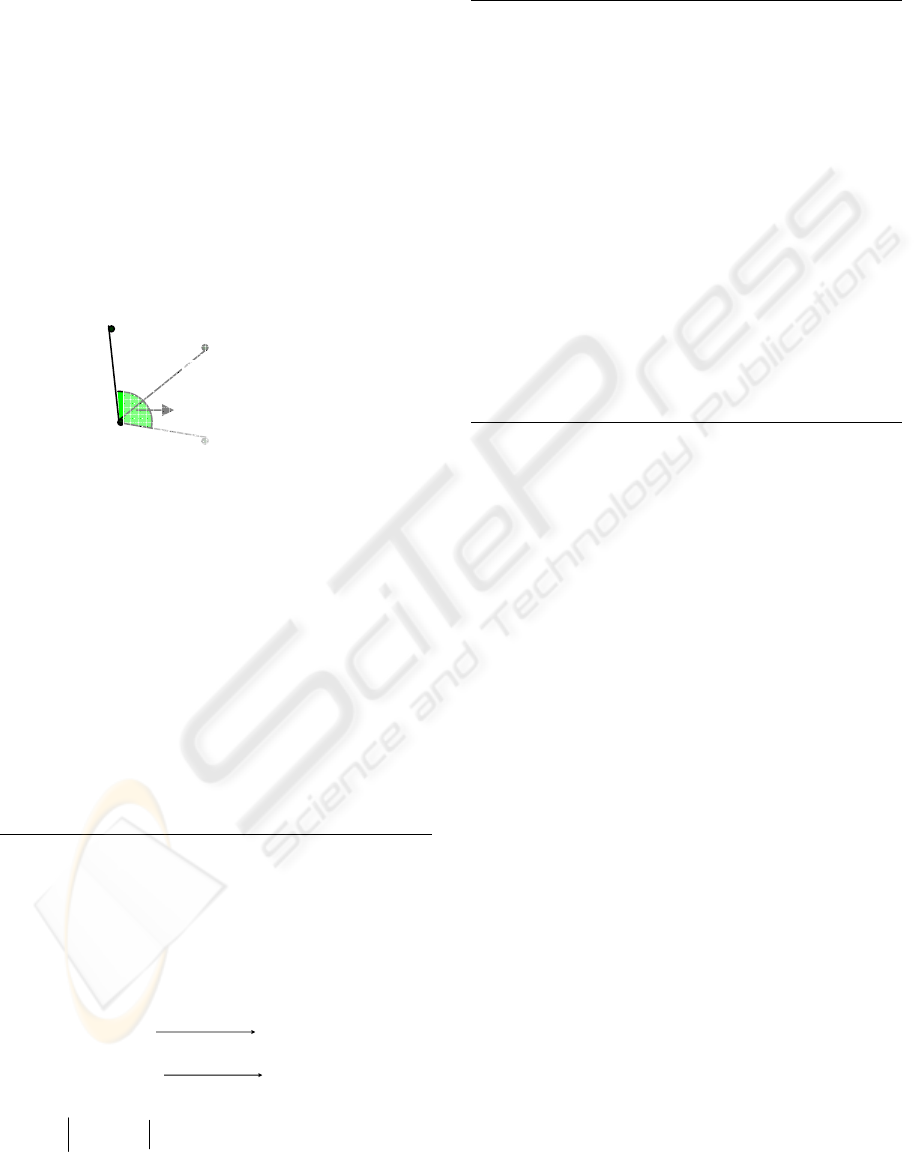
Figure 5: Controlling sampling domain with angular
parameter.
Definition 3: given
free
CS
of the configuration
space. For a node
near
v and the goal
configuration
goal
v
. The Angular Domain is defined
as the intersection between
free
CS
and the samples
candidate who satisfies the control sampling
algorithm (in green colour Figure 5) defined below:
SELECT_NEIGHBOR (
)q
1) Repeat
2) Pick
rand
q at random from a uniform distribution
over
free
CS
according to a suitable threshold
distance
R
from
q
.
3)
),(
1
OxqqAngle
rand
← θ
4)
),(
2
OxqqAngle
goal
← θ
5) If
param
θθθ ≤−
21
6) Return
rand
q
7) End
BUILD PLANNER
)(
init
q
1)
initnear
qq
=
2) Repeat
3)
)(_
nearrand
qNeighborSelectq
←
4) ),(_
nearrands
qqionConfiguratStoppq
←
5)
)(_
s
qvertexadd
6) )(_
snear
qqedgeadd
7) If CONNECT
)(
sgoal
qq
8) Return path
9) Else
snear
qq
=
10) End repeat
Figure 6: The control sampling algorithm and the Angular
Domain planner in 2D environment.
3.4 Implementation
Point robot: for those types of robots we have 2
translational degrees of freedom. The configuration
of the robot is a vector
T
yxq ),(= . Once a random
configuration
rand
q is sampled according to
threshold distance
R
which is computed by the
Euclidean distance in
2
R
, the select neighbour
algorithm computes two quantities.
1
θ
represents
the angle between the vector
⎯→⎯
rand
qq(
)and the
horizontal axis in 2D workspace in which
q
is the
current configuration in the tree and
rand
q the
sample candidate for interpolation.
2
θ
is the angle
between the vector
⎯→⎯
)(
goal
qq
and also the horizontal
axis in 2D workspace see figure (5). If the absolute
value of the difference between these two quantities
is less or equal to some chosen
prameter
θ
value, the
edge
)(
rand
qq is created. The local planner
performs the interpolation and checks for collision
free each placement.
near
q
1rand
q
param
θ
goal
q
A NEW PROBABILISTIC PATH PLANNER - For Mobile Robots Comparison with the Basic RRT Planner
405

3.5 Computational Analysis
The running time T for an RRT planner is given by
the relation:
conconnodenode
NTNTT ×+×= (3)
:
node
T The average cost of sampling one node
node
N : The number of the nodes in the tree
con
T : The average cost of checking collision-free
connections between two nodes.
con
N : The number of calls to check collision-free
connections between two nodes.
For the basic RRT algorithm collision checks
operation is performed twice. First in line 5 Figure 2
to interpolate
rand
q and
near
q . The second collision
detection is made to see if the goal configuration is
reached or not. The Angular Domain planner
performs also the collision detection operation twice.
First to compute
s
q in line 4 figure 6 in the structure
of the Angular Domain planner. The second time in
Line 7 to interpolate
s
q to
goal
q
. The difference
between the two approaches is in the number of
placements we check for collision indeed; since we
use the incremental method to check whether a
placement is free or not, given two nodes the
number of placements we check represent
con
N .
Recall that between two nodes we interpolate
until
s
q , we are able to reduce
con
N comparing with
the RRT which checks for all the placements
between two node
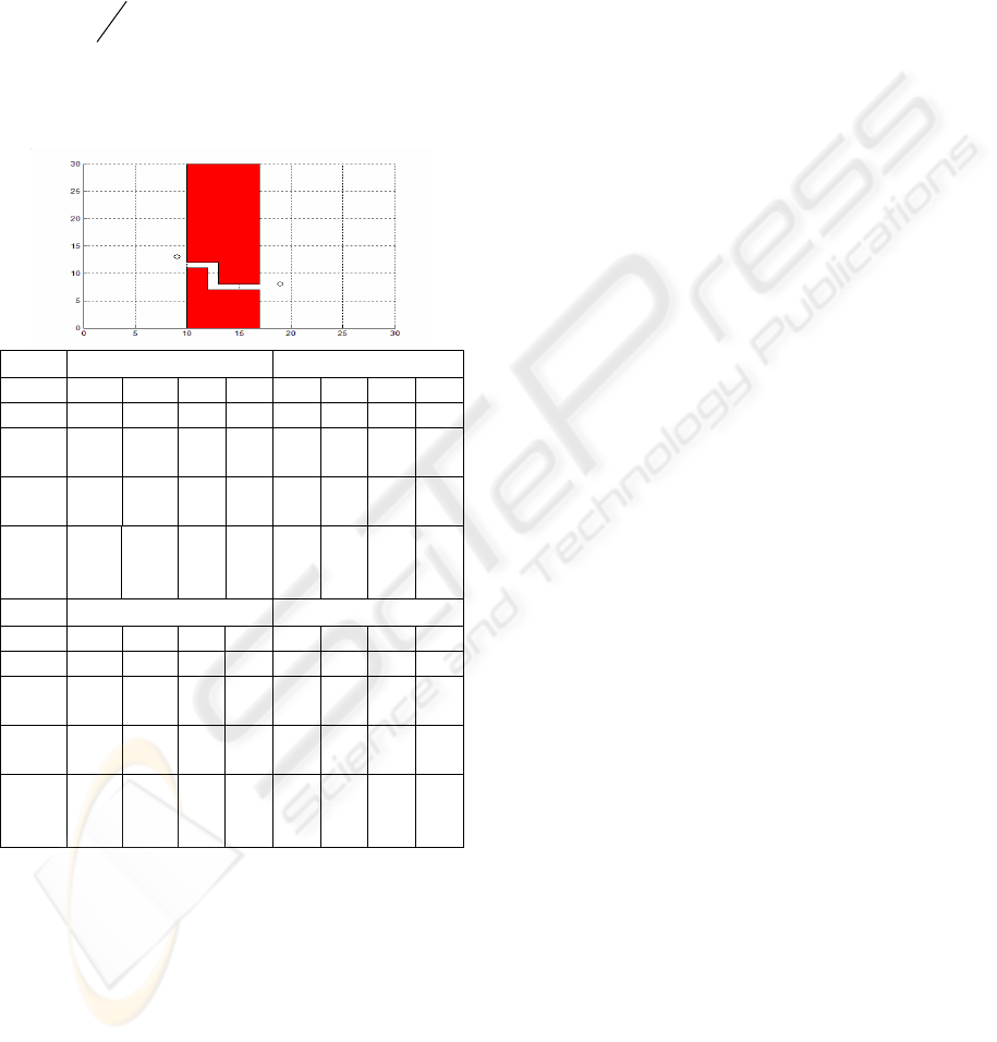
3.6 Simulations
The Angular Domain RRT planner and the Basic
RRT planner were simulated under Matlab
environment. Simulations were performed on a 3.2
GHZ Pentium IV. For each example the
performance of for the mono directional RRT
algorithms and the Angular Domain RRT algorithms
are compared. Comparison is performed in terms of
the running time and the number of collision checks
made by both planners.
Angular domain
planner
RRT
planner
Time (1)
(s)
1.7500 2.3408
Num.nodes
N (1) in the tree
7 30
mill
n (1)
191 46
CD calls
(1)
4279 3784
Success
rate (%) (1)
100% 30%
Time (2)
(s)
2.214 6.86
Num.nodes
N (2)
15 80
mill
n (2)
238 149
CD calls
(2)
3967 11479
Success
rate (%) (2)
100% 0%
best worst Time (3)
(s)
4.0160se 46.1250
10.4220
best worst Num.nodes
N (3)
15 20
100
best worst
mill
n (3)
280 257853
202
best worst CD calls
(3)
7297 91850
15884
Success
rate (%) (3)
100% 0%
Figure 7: simulations results for the environment in
Figure.
The table Figure 7 shows the result obtained for
an environment with a classic narrow passage the
results are an averaged of 50 runs over the three
environment. The success rate characterizes the
performance of both planners to find the solution
path. The first observation we made on these results
is that as the width of the narrow passage became
smaller the performance of the basic RRT planner
ICINCO 2007 - International Conference on Informatics in Control, Automation and Robotics
406

deteriorate quickly (see the success rate lines for the
three environments).the deterioration of the
performance is explained by the fact that the size of
the free space is considerably larger than the narrow
opening in the three environments We make the
second observation on the third environment, as it
was mentioned in the computational analysis section
the threshold distance and the angular parameter (set
to 10 and
2
π
) must be chosen carefully. We can
see that
mill
n has a very large value (see Line14
Figure 7) leading to increase the total running time
of the algorithm in the worst case.
Angular domain RRT N=5
R
5 10 20 30 5 10 20 30
time
3.81 4.17 2.96 2.23 0.46 0.32 0.34 0.53
CD
calls
8098 7081
3369 2113 571 554 579 565
mill
n
930
1
431 868 69 18 5 6 6
Succ
es
(%)
100 100 100 100 0 0 0 0
RRT N=80 RRT N=200
R
5 10 20 30 5 10 20 30
time
3.71 3.92 2.96 4.12 24 24 25 25
CD
calls
5
597
5
838
5884 6045 22335 23504 23892 23193
mill
n
75 66 64 68 293 297 283 285
Succ
es
(%)
0 0 0 0 0 0 0 0
Figure 8: simulation results for the environment with
different N (the maximum number of the node for RRT).
The simulation results demonstrate the efficiency
of the Angular Domain planner. We take different
values of
R
, it appears that the optimal threshold
distance for the environment figure 8 is 30; it gives
also the smallest running time. Note that for a small
threshold distance (5 and 10) we can see that
mill
n
is big leading to increase the total running time of
our algorithm. Therefore for a given problem the
balance between too small or to large value for the
threshold distance can be difficult to find indeed; too
small value may increase dramatically
mill
n
and by
the way the total running time
T
in the other hand
too large value may potentially add many nodes in
the open free space while we need much nodes in
the narrow passage.
4 CONCLUSIONS AND FUTURE
WORK
There are to ways to improve the current work. First
the threshold distance and the angular parameter are
chosen manually a promising approach is to adjust
these two parameters through on line learning. The
tuning of these two parameters will be obviously
based on the position of the obstacles in the
workspace leading to get an efficient planner for
different kinds of obstacles.
Another important direction is to apply this
frame work for other constrained motion planning
problems such articulated robot
REFERENCES
J. H. Reif, “Complexity of the mover’s problem and
generalizations,” in Proceedings of the 20
th
IEEE
Symposium on Foundations of Computer Science,
1979, pp. 421-427.
P. Svestka, Robot motion planning using probabilistic
roadmaps. Ph.D Thesis, Utrecht University, 1997.
L. E.Kavraki, J.-C.Latombe, Randomized preprocessing of
configuration space for fast path planning, In:IEEE
Int Conf On Robotics and Automation,1994,pp.2138-
2145.
S. M. La Valle Rapidly-exploring random trees: A new
tool for path planning. TR 98-11, Computer Science
Dept., Iowa State University, Oct. 1998.
E. Ferré and J.-P. Laumond An iterative diffusion method
for part disassembly. In IEEE Int.Conf .Robot.&
Autom.,2004
A. Yershova and S. M. LaValle. planning for closed
chains without inverse kinematics, in: IEEE Conf On
Robotics and Automation, 2007 to appear
F. Lamiraux, E.Ferre, and E. Vallee. kinodynamic motion
planning: connecting exploration trees using
trajectory optimization methods. In IEEE In Conf
Robot & Autom, pages 3987-3992, 2004.
Sofiane Ahmed Ali, Eric Vasselin and Alain Faure. “A
new Hybrid sampling strategy for PRM planners to
address narrow passages problem”. In Proceedings
3rd International Conference on Informatics in
Control, Automation and Robotics (ICINCO), 2006.
A NEW PROBABILISTIC PATH PLANNER - For Mobile Robots Comparison with the Basic RRT Planner
407