
NONLINEAR MODEL PREDICTIVE CONTROL OF A LINEAR
AXIS BASED ON PNEUMATIC MUSCLES
Harald Aschemann and Dominik Schindele
Chair of Mechatronics, University of Rostock, Justus-von-Liebig-Weg 6, D-18059 Rostock, Germany
Keywords:
Mechatronics, predictive control, flatness-based methods, pneumatic muscle.
Abstract:
This paper presents a nonlinear optimal control scheme for a mechatronic system that consists of a guided
carriage and an antagonistic pair of pneumatic muscles as actuators. Modelling leads to a system of nonlinear
differential equations including polynomial approximations of the volume characteristic as well as the force
characteristic of the pneumatic muscles. The proposed control has a cascade structure: the nonlinear norm-
optimal control of both pneumatic muscle pressures is based on an approximative solution of the corresponding
HJB-equation, whereas the outer control loop involves a multivariable NMPC of the carriage position and the
mean internal pressure of the pneumatic muscles. To improve the tracking behaviour, the feedback control
loops are extended with nonlinear feedforward control based on differential flatness. Remaining model un-
certainties as well as nonlinear friction can be counteracted by an observer-based disturbance compensation.
Experimental results from an implementation on a test rig show an excellent control performance.
1 INTRODUCTION
Pneumatic muscle actuators are tension actuators con-
sisting of a fiber-reinforced vulcanised rubber tubing
with connection flanges at both ends. Due to a spe-
cial fiber arrangement, the pneumatical muscle con-
tracts with increasing internal pressure. This effect
can be used for actuation purposes. Pneumatic mus-
cles offer major advantages in comparison to classi-
cal pneumatic cylinders: significantly less weight, no
stick-slip effects, insensitivity to dirty working envi-
ronment, and a larger maximum force. The nonlinear
characteristics of the muscle, however, demand for
nonlinear control, e.g. flatness-based control (Fliess
et al., 1995), (Aschemann and Hofer, 2004). For the
practical investigation of control approaches the test
rig shown in figure 1 has been built. Two guide-
ways with roller bearing units allow for rectilinear
movements of a carriage with small nonlinear friction
forces. On opposite sides of the carriage, pneumatic
muscles are arranged in an antagonistic configuration
between the carriage and the rigid frame. The mass
flow of air of each pneumatic muscle is controlled by
means of a proportional valve. The in-flowing air is
provided at a maximum pressure of 7 bar, whereas
the out-flowing air is discharged at atmospheric pres-
sure, i.e. 1 bar. Pressure declines in the case of large
commanded mass flows are counteracted by using
compensator reservoirs, which maintain an approxi-
mately constant pressure supply level for each pneu-
matic muscle. Similarly, an additional compensator
reservoir in combination with a sound absorber re-
duces the noise caused by discharged air. The pa-
per is structured as follows: first, the modelling of the
mechatronic system is addressed. Second, a nonlinear
cascade control scheme is proposed: nonlinear H
2
-
optimal control loops, which can be realised with high
bandwidth, guarantee a specified internal pressure in
each pneumatic muscle (Aschemann et al., 2006).
The outer control loop involves nonlinear model pre-
dictive trajectory control of the carriage position and
the mean muscle pressure as controlled variables and
provides the reference pressures for the inner pressure
control loops. Aiming at good tracking behaviour,
feedforward control based on differential flatness is
considered in the control structure as well. A distur-
bance force resulting from remaining modelling er-
rors w.r.t. the force characteristic of the pneumatic
92
Aschemann H. and Schindele D. (2007).
NONLINEAR MODEL PREDICTIVE CONTROL OF A LINEAR AXIS BASED ON PNEUMATIC MUSCLES.
In Proceedings of the Fourth International Conference on Informatics in Control, Automation and Robotics, pages 92-99
DOI: 10.5220/0001649200920099
Copyright
c
SciTePress
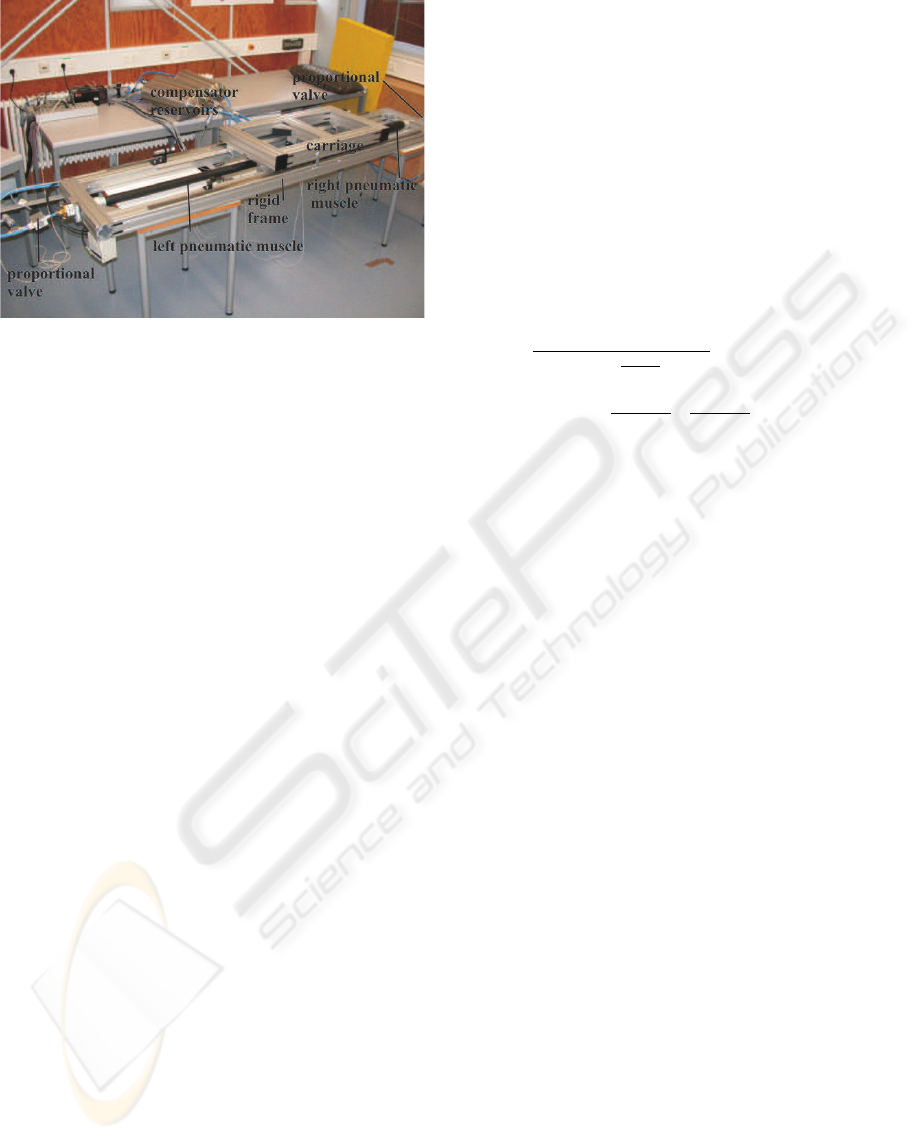
Figure 1: Linear axis test rig.
muscles as well as the friction characteristic of the
carriage is estimated by a reduced-order disturbance
observer and used for compensation in the nonlinear
control scheme. By this, desired trajectories for both
carriage position and mean pressure can be tracked
with high accuracy as shown by experimental results
from an implementation at the test rig.
2 SYSTEM MODELLING
As for modelling, the mechatronic system is divided
in a pneumatic subsystem and a mechanical subsys-
tem, which are coupled by the tension forces of the
two pneumatic muscles. In contrast to the model
of (Carbonell et al., 2001) the dynamics of the pneu-
matic subsystem is also included. The tension force
F
Mi
≥ 0 and the volume V
Mi
of the pneumatic mus-
cle i, i = r, l, nonlinearly depend on the according
internal pressure p
Mi
as well as the contraction length
∆ℓ
Mi
. The origin of the generalised coordinate x
S
(t)
of the carriage is defined as the position where the
right muscle is fully contracted. Then, the constraints
∆ℓ
Ml
(x
S
) = x
S
, ∆ℓ
Mr
(x
S
) = ∆ℓ
M, max
− x
S
(1)
hold. Consequently, the contraction lengths of both
pneumatic muscles are related to the carriage posi-
tion.
2.1 Modelling of the Pneumatic
Subsystem
The dynamics of the internal muscle pressure follows
directly from a mass flow balance in combination with
the energy equation for the compressed air in the mus-
cle. As the internal muscle pressure is limited by
a maximum value of p
Mi,max
= 7 bar, the ideal
gas equation represents an accurate description of the
thermodynamic behaviour. The thermodynamic pro-
cess is modelled as a polytropic change of state with
n = 1.26 as identified polytropic exponent. The iden-
tified volume characteristic of the pneumatic muscle
can be described by a polynomial function
V
Mi
(∆ℓ
Mi
, p
Mi
) =
3
X
j=0
a
j
· ∆ℓ
j
Mi
·
1
X
k=0
b
k
· p
k
Mi
.
(2)
with the contraction length ∆ℓ
Mi
and the muscle
pressure p
Mi
. The resulting state equation for the in-
ternal muscle pressure in the muscle i is given by
˙p
Mi
=
n
V
Mi
+ n ·
∂V
Mi
∂p
Mi
· p
Mi
[R
L
· ϑ(·) · ˙m
Mi
−
∂V
Mi
∂∆ℓ
Mi
·
∂∆ℓ
Mi
∂x
S
· p
Mi
· ˙x
S
, (3)
where R
L
denotes the gas constant of air. The func-
tion ϑ(n, T
S
, T
Mi
, sign( ˙m
Mi
)), which depends on
the polytropic exponent n, the air supply tempera-
ture T
S
, the internal temperature T
Mi
, and the sign
of the mass flow rate ˙m
Mi
, can be approximated with
good accuracy by the constant temperature T
0
of the
ambiance. Thereby, temperature measurements can
be avoided, and the implementational effort is signif-
icantly reduced.
2.2 Modelling of the Mechanical
Subsystem
The mechanical subsystem is related to the motion of
the carriage with mass m
S
= 30 kg on its guideways.
The nonlinear force characteristic F
Mi
(p
Mi
, ∆ℓ
Mi
)
of a pneumatic muscle represents the resulting ten-
sion force for given internal pressure p
Mi
as well as
given contraction length ∆ℓ
Mi
. It has been identified
by static measurements and, then, approximated by a
polynomial description
F
Mi
(∆ℓ
Mi
, p
Mi
) =
¯
F
Mi
(∆ℓ
Mi
)·p
Mi
−f
Mi
(∆ℓ
Mi
).
(4)
The equation of motion follows directly from New-
ton’s second law as a second order differential equa-
tion for the carriage position
m
S
· ¨x
S
= F
Ml
(·) − F
Mr
(·) − F
U
. (5)
At this, remaining model uncertainties are taken into
account by the disturbance force F
U
. These uncer-
tainties stem from approximation errors concerning
the static muscle force characteristics, non-modelled
viscoelastic effects of the vulcanised rubber material,
and viscous damping as well as friction forces acting
on the carriage.
NONLINEAR MODEL PREDICTIVE CONTROL OF A LINEAR AXIS BASED ON PNEUMATIC MUSCLES
93

3 NORM-OPTIMAL CONTROL
OF THE MUSCLE PRESSURES
In the sequel, the nonlinear norm-optimal control de-
sign is presented (Lukes, 1969). The design approach
applies to the following class of systems
˙
x(t) = Ax(t) + Bu(t) + f (x(t), u(t)) ,
y = h (x(t), u(t)) = Cx(t) + Du(t),
(6)
with the affine control input u ∈ U ⊂ R
m
, the
state vector x ∈ X ⊂ R
n
and the output vector
y ∈ Y ⊂ R
p
. The non-linearity f (x, u) can be
stated as f (x, u) = f
(2)
(x, u) + f
(3)
(x, u) + ...,
where f
(m)
(x, u) denotes a polynomial of degree m
in terms of x and u. The H
2
-optimal control aims at
calculating a nonlinear state feedback law u(x) with
u(0) = 0 such that the nonlinear cost function
J(u) = inf
u∈L
m
2
[0,∞)
Z
∞
0
Λ
2
(x, u)dt (7)
with
Λ
2
(x, u) =
1
2
y
T
Qy + u
T
Ru
+ l(x, u)
=
1
2
x
T
˜
Qx +
1
2
u
T
˜
Ru + x
T
N u + l(x, u)
(8)
is minimized. The symmetric, positive definite
weighting matrix Q = Q
T
> 0 accounts for the
output variables, whereas the symmetric, positive
definite weighting matrix R regards the control in-
puts. The nonlinear term l(x, u) = l
(3)
(x, u) +
l
(4)
(x, u) + ... consists of expressions of third or
higher degrees in terms of x and u. In the case of
l(x, u) = 0 the cost function becomes quadratic. The
solution of the above stated optimization problem is
given by the positive definite solution J (x) : X →
R
+
of a nonlinear partial differential equation, the
Hamilton-Jacobi-Bellman-equation (HJB-equation)
min
u
H (x, J
x
(x), u) = 0, (9)
with the corresponding Hamiltonian
H = J
x
(x) [Ax + Bu + f(x, u)] + Λ
2
(x, u).
(10)
In the considered unconstrained case, the optimal so-
lution u
∗
is obtained from the stationary condition
H
u
= 0. Consequently, the two equations
H =J
x
(x) [Ax + Bu + f(x, u)] +
1
2
x
T
˜
Qx
+ x
T
Nu +
1
2
u
T
˜
Ru + l(x, u) = 0
(11)
and
H
u
= J
x
(x) (B + f
u
(x, u)) + x
T
N
+ u
T
˜
R + l
u
(x, u) = 0
(12)
need to be solved. These equations are approximately
solved by an approach according to (Lukes, 1969)
based on power series expansions of the involved non-
linear functions . The gradient of the optimal solution
J (x) and the control law are recursively determined
by a step-by-step solution of both equations for a con-
sidered degree k of the according polynomials in x
and u.
3.1 Feedback Control Design
The control design for both internal muscle pressures
is identical (Aschemann et al., 2006). For the sake of
simplicity, the internal muscle pressure as state vari-
able is denoted as x := p
Mi
, i = {r, l}, and the con-
trol input as u := u
pi
= R
L
· T
0
· ˙m
Mi
. Then, the
state equation (3) can be rewritten as
˙x =
n ·
u − k
1
(x
S
, ˙x
S
) · x − k
2
(x
S
, ˙x
S
) · x
2
k
3
(x
S
) + k
4
(x
S
) · x
,
(13)
According to the continuous dependence of the coef-
ficients k
i
(x
S
, ˙x
S
) on x
S
and ˙x
S
, the resulting feed-
back control law is adapted by gain-scheduling. Af-
ter a truncated Taylor series expansion with respect to
x = p
Mi
, the nonlinear state space description for the
muscles pressure becomes
˙x = a(u) + b(u) · x + c(u) · x
2
+ d(u) · x
3
+ e(u) · x
4
+ g(u) · x
5
,
y = x,
(14)
The quadratic cost function with l(x, u) = 0 is given
by
J(u) =
1
2
Z
∞
0
q
p
x
2
+ r
p
u
2
dt, (15)
where the scalar r
p
serves as a weighting factor for
the input variable u = u
pi
and the scalar q
p
as weight-
ing factor for the state variable, i.e. the muscle pres-
sure x = p
Mi
. The H
2
-optimal control laws for these
fast inner control loops are calculated up to the degree
k = 3, i.e. u
pi,F B
(x) =
P
3
j=1
u
0(j)
. The resulting
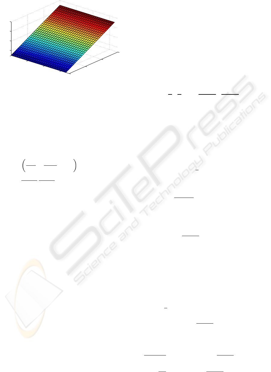
nonlinear feedback control law u
pl,F B
(p
Ml
, x
S
, ˙x
S
)
for the left muscle is depicted in Fig. 2 for ˙x
S
=
0.1 m/s. Obviously, the linear part dominates the non-
linear terms.
3.2 Feedforward Control Design
As for feedforward control design, differential flat-
ness can be exploited for the system under consid-
eration (Fliess et al., 1995). The muscle pressure
ICINCO 2007 - International Conference on Informatics in Control, Automation and Robotics
94
1
3
5
7
0
0.1
0.2
0.3
−6
−4
−2
0
x 10
4
p
Ml
in N/m
2
x 10
5
x
S
in m
u
pl,FB
in J/s
Figure 2: Nonlinear H
2
-optimal feedback control law
u
pl,F B
(p
Ml
, x
S
, ˙x
S
) for the left pneumatic muscle for the
gain-scheduling parameters x
S
and ˙x
S
= 0.1 m/s.
y = p
Mi
, i = {r, l}, obviously represents a flat out-
put of the corresponding inner control loop. Evaluat-
ing the state equation (3) for the muscle pressure with
desired values for the flat output y
d
= p
Mid
as well
as its time derivative ˙y
p
= ˙p
Mid
and solving for the
feedforward control part u
pi,F F
result in
u
pi,F F
=
V
Mi
n
+
∂V
Mi
∂p
Mi
· p
Mid
˙p
Mid
+
∂V
Mi
∂∆l
Mi
∂∆l
Mi
∂x
S
· ˙x
S
· p
Mid
− u
pi,F B
(p
Mid
).
(16)
Note that the measured values x
S
and ˙x
S
are used for
a gain-scheduled adaptation of the feedforward con-
trol law. As a result, the overall control law for the
inner control loops becomes u
pi
= u
pi,F F
+ u
pi,F B
.
4 NONLINEAR MPC
The main idea of the control approach consists in a
minimization of a future tracking error in terms of the
predicted state vector based on the actual state and
the desired state vector resulting from trajectory plan-
ning (Lizarralde et al., 1999), (Jung and Wen, 2004).
The minimization is achieved by repeated approxi-
mate numerical optimization in each time step, in
the given case using the Newton-Raphson technique.
The optimization is initialised in each time step with
the optimization result of the preceeding time step in
form of the input vector. The NMPC-algorithm is
based on the following nonlinear discrete-time state
space representation
x
k+1
= f (x
k
, u
k
) , y
k
= h(x
k
, u
k
) , (17)
with the state vector x
k
∈ R
n
, the control input u
k
∈
R
m
and the output vector y
k
∈ R
p
. The constant M
specifies the prediction horizon T
P
as a multiple of
the sampling time t
s
, i.e. T
P
= M · t
s
. The predicted
input vector at time k becomes
u
k,M
=
u
(k)
1
T
, ..., u
(k)
M
T
T
, (18)
with u
k,M
∈ R
m·M
. The predicted state vector at
the end of the prediction horizon φ
M
(x
k
, u
k,M
) is
obtained by repeated substitution of k by k + 1 in the
discrete-time state equation (17)
x
k+2
= f (x
k+1
, u
k+1
) = f(f(x
k
, u
k
), u
k+1
)
.
.
.
x
k+M
= f (· · · f
|
{z }
M
(x
k
, u
k
), · · · , u
k+M −1
|
{z }
M
)
= φ
M
(x
k
, u
k,M
) .
(19)
The difference of φ
M
(x
k
, u
k,M
) and the desired
state vector x
d
leads to the final control error
e
M,k
= φ
M
(x
k
, u
k,M
) − x
d
, (20)
i.e. to the control error at the end of the prediction
horizon. The cost function to be minimized follows
as
J
MP C
=
1
2
· e
T
M,k
e
M,k
, (21)
and, hence, the necessary condition for an extremum
can be stated as
∂J
MP C
∂e
M,k
= e
M,k
!
= 0 . (22)
A Taylor-series expansion of (22) at u
k,M
in the
neighbourhood of the optimal solution leads to the
following system of equations
0 = e
M,k
+
∂φ
M
∂u
k,M
∆u
k,M
+ T.h.O. (23)
The vector ∆u
k,M
denotes the difference which has
to be added to the input vector u
k,M
to obtain the
optimal solution. The n equations (23) represent an
under-determined set of equations with m · M un-
knowns having an infinite number of solutions. A
unique solution for ∆u
k,M
can be determined by
solving the following L
2
-optimization problem with
(23) as side condition
J =
1
2
· ∆u
T
k,M
∆u
k,M
+ λ
T
e
M,k
+
∂φ
M
∂u
k,M
∆u
k,M
.
(24)
Consequently, the necessary conditions can be stated
as
∂J
∂∆u
k,M
!
= 0 = ∆u
k,M
+
∂φ
M
∂u
k,M
T
λ,
∂J
∂λ
!
= 0 = e
M,k
+
∂φ
M
∂u
k,M
∆u
k,M
,
(25)
NONLINEAR MODEL PREDICTIVE CONTROL OF A LINEAR AXIS BASED ON PNEUMATIC MUSCLES
95

which leads to e
M,k
:
e
M,k
=
∂φ
M
∂u
k,M
∂φ
M
u
k,M
T
|
{z }
S(φ
M
,u
k,M
)
λ . (26)
If the matrix S (φ
M
, u
k,M
) is invertible, the vector λ
can be calculated
λ = S
−1
(φ
M
, u
k,M
) e
M,k
. (27)
An almost singular matrix S (φ
M
, u
k,M
) can be
treated by a modification of (27)
λ = [µI + S (φ
M
, u
k,M
)]
−1
e
M,k
, (28)
where I denotes the unity matrix. The regularisation
parameter µ > 0 in (28) may be chosen constant or
may be calculated by a sophisticated algorithm. The
latter solution improves the convergence of the op-
timization but increases, however, the computational
complexity. Solving (25) for ∆u
k,M
and inserting
λ according to (27) or (28), directly leads to the L
2
-
optimal solution
∆u
k,M
= −
∂φ
M
∂u
k,M
T
S
−1
(φ
M
, u
k,M
) e
M,k
= −
∂φ
M
∂u
k,M
†
e
M,k
.
(29)
Here,
∂φ
M
∂u
k,M
†
denotes the Moore-Penrose pseudo
inverse of
∂φ
M
∂u
k,M
. The overall NMPC-algorithm can
be described as follows:
Choice of the initial input vector u
0,M
at time k = 0,
e.g. u
0,M
= 0, and repetition of steps a) - c) at each
sampling time k ≥ 0:
a) Calculation of an improved input vector v
k,M
ac-
cording to
v
k,M
= u
k,M
− η
k
∂φ
M
∂u
k,M
†
e
M,k
. (30)
The step width η
k
can be determined with, e.g.,
the Armijo-rule.
b) For the calculation of u
k+1,M
the elements of the
vector v
k,M
have to be shifted by m elements and
the steady-state input vector u
d
corresponding to
the final state has to be inserted at the end u
d
u
k+1,M
=
0
(m(M−1)×m)
I
(m)
u
d
+
0
(m(M−1)×m)
I
(m(M−1))
0
m×m
0
(m×m(M−1))
v
k,M
.
(31)
In general, the steady-state control input u
d
can
be computed from
x
d
= f (x
d
, u
d
). (32)
For differentially flat systems the desired input
vector u
d
is given by the inverse dynamics and
can be stated as a function of the flat outputs and
their time derivatives.
c) The first m elements of the improved input vector
v
k,M
are applied as control input at time k
u
k
=
I
(m)
0
(m×m(M−1))
v
k,M
. (33)
In the proposed algorithm only one iteration is per-
formed per time step. A similar approach using sev-
eral iteration steps is described in (Weidemann et al.,
2004).
4.1 Numerical Calculations
The analytical computation of the Jacobian
∂φ
M
∂u
k,M
be-
comes increasingly complex for larger values of M .
Therefore, a numerical approach is preferred taking
advantage of the chain rule with i = 0, ..., M − 1
∂φ
M
∂u
(k)
i+1
=
∂φ
M
∂x
k+M −1
·
∂x
k+M −1
∂x
k+M −2
· · · ·
·
∂x
k+i+2
∂x
k+i+1
·
∂x
k+i+1
∂u
(k)
i+1
.
(34)
Introducing the abbreviations
A
i
:=
∂x
k+i+1
∂x
k+i
=
∂f
∂x
x
k+i
, u
(k)
i+1
, (35)
B
i
:=
∂x
k+i+1
∂u
(k)
i+1
=
∂f
∂u
x
k+i
, u
(k)
i+1
, (36)
the Jacobian can be computed as follows
∂φ
M
∂u
k,M
= [A
M−1
A
M−2
· · · A
1
B
0
,
A
M−1
· · · A
2
B
1
, ..., A
M−1
B
M−2
, B
M−1
] .
(37)
For the inversion of the symmetric and positive def-
inite matrix S (φ
M
, u
k,M
) =
∂φ
M
∂u
k,M
∂φ
M
∂u
k,M
T
the
Cholesky-decomposition has proved advantageous in
terms of computational effort.
4.2 Choice of the Nmpc Design
Parameters
The most important NMPC design parameter is the
prediction horizon T
P
, which is given as the prod-
uct of the sampling time t
s
and the constant value
ICINCO 2007 - International Conference on Informatics in Control, Automation and Robotics
96
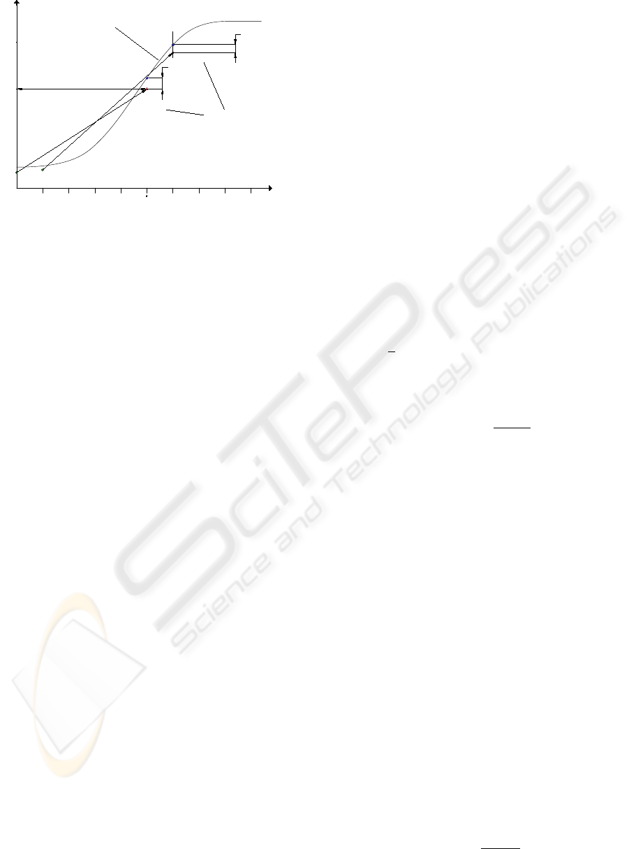
T
P
e
M,0
x
0
φ
M
(x , u )
0
0,M
Desired Trajectory
x
t
t
s
φ
M
(x , u )
1
1,M
x
1
e
M,1
t
s
M
Predicted state
x
d,0
x
d,1
Figure 3: Design parameters.
M. Large values of T
P
lead to a slow and smooth
transient behaviour and result in a robust and stable
control loop. For fast trajectory tracking, however,
a smaller value T
P
is desirable concerning a small
tracking error. The choice of the sampling time t
s
is crucial as well: a small sampling time is neces-
sary regarding discretization error and stability; how-
ever, the NMPC-algorithm has to be evaluated in real-
time within the sampling inverval. Furthermore, the
smaller t
s
, the larger becomes M for a given pre-
diction horizon, which in turn increases the compu-
tational complexity of the optimization step. Conse-
quently, a system-specific trade-off has to be made
for the choice of M and t
s
. This paper follows the
moving horizon approach with a constant prediction
horizon and, hence, a constant dimension m · M of
the corresponding optimization problem in constrast
to the shrinking horizon approach (Weidemann et al.,
2004).
4.3 Input Constraints
One major advantage of predictive control is the pos-
sibility to easily account for input constraints, which
are present in almost all control applications. To this
end, the cost function can be extended with a corre-
sponding term
h(u
(k)
j
) =
0 u
min
≤ u
(k)
j
≤ u
max
g
1
(u
(k)
j
) for u
(k)
j
> u
max
g
2
(u
(k)
j
) u
(k)
j
< u
min
,
(38)
which has to be evaluated componentwise, i.e. for
each input variable at each sampling time. Thus,
the contribution of the additional input constraints
depending on u
k,M
is given by
z(u
k,M
) =
M
X
j=1
h(u
(k)
j
) (39)
Instead of e
M,k
the vector
h
e
T
M,k
, z
i
T
has to be min-
imized in the NMPC-algorithm.
5 MODIFICATIONS OF THE
ALGORITHM
To improve trajectory tracking behaviour, the NMPC-
algorithm can be modified as follows:
(1) Instead of a minimization of the control error at
the end of the prediction horizon given by the dif-
ference of the predicted value φ
M
(x
k
, u
k,M
) and
the according reference value x
d
, the minimization
could take into account additional predicted errors
e
Mi,k
= φ
Mi
(x
k
, u
k,M i
) − x
di
, i ∈ N , Mi < M .
Thus, the cost function (21) is modified as follows
J
MP C
=
1
2
(e
T
M1,k
e
M1,k
+ ... + e
T
M,k
e
M,k
) (40)
The required values φ
Mi
are already known from
the calculation of φ
M
and, hence, do not further
increase the computational effort. Unfortunately,
the additional computation of
∂φ
Mi
∂u
Mi,k
as well as the
increased dimension of the matrix to be inverted
S(φ
M1
, ..., φ
M
, u
k,M 1
, ..., u
k,M
) have a significant
impact on the computation time. Therefore, the num-
ber of expressions in the cost function should be kept
as small as possible, especially in the given case of a
fast higher-dimensional system.
(2) A further improvement of the trajectory tracking
behaviour can be achieved if an input vector resulting
from an inverse system model is used as initial vector
for the subsequent optimization step instead of the last
input vector. Since the system under consideration is
differentially flat (Aschemann and Hofer, 2004), the
required ideal control input can be derived for a given
reference trajectory. The slightly modified algorithm
can be stated as follows
a) Calculation of the ideal input vector u
(d)
k,M
by
evaluating an inverse system model with the spec-
ified reference trajectory as well as a certain num-
ber β ∈ N of its time derivatives
u
(d)
k,M
= u
(d)
k,M
y
d
, ˙y
d
, ...,
(β)
y
d
. (41)
b) Calculation of the improved input vector v
k,M
based on the equation
v
k,M
= u
(d)
k,M
− η
k
∂φ
M
∂u
k,M
†
e
M,k
. (42)
NONLINEAR MODEL PREDICTIVE CONTROL OF A LINEAR AXIS BASED ON PNEUMATIC MUSCLES
97

c) Application of the first m elements of v
k,M
to the
process
u
k
=
I
(m)
0
(m×m(M−1))
v
k,M
. (43)
If the reference trajectory is known in advance, the ac-
cording reference input vector u
(d)
k,M
can be computed
offline. Consequently, the online computational time
remains unaffected. Of course, all the proposed mod-
ifications could be combined.
5.1 Nmpc of the Carriage Position
The state space representation for the position control
design can be directly derived from the equation of
motion for the carriage
˙
x =
˙x
S
¨x
S
=
˙x
S
F
Ml
(x
S
,p
Ml
)−F
Mr
(x
S
,p
Mr
)
m
S
.
(44)
The carriage position x
S
and the carriage velocity ˙x
S
represent the state variables, whereas the input vector
consists of the left as well as the right internal muscle
pressure, p
Ml
and p
Mr
. The discrete-time representa-
tion of the continous-time system (44) is obtained by
Euler discretisation
x
k+1
= x
k
+ t
s
· f(x
k
, u
k
) (45)
Using this simple discretisation method, the compu-
tational effort for the NMPC-algorithm can be kept
acceptable. Furthermore, no significant improvement
was obtained for the given system with the Heun dis-
cretisation method because of the small sampling time
t
s
= 5 ms. Only in the case of large sampling times,
e.g. t
s
> 20 ms, the increased computational effort
caused by a sophisticated time discretisation method
is advantageous. Then, the smaller discretisation er-
ror allows for less time integration steps for a speci-
fied prediction horizon, i.e. a smaller number M. As a
result, the smaller number of time steps can overcom-
pensate the larger effort necessary for a single time
step. The flat output variables of (44) are given by
y =
x
S
p
M
=
x
S
1
2
· (p
Ml
+ p
Mr
)
. (46)
Using the desired trajectories for the carriage position
x
Sd
and the mean muscle pressure p
Md
, the corre-
sponding desired input values result in
u
d
=
p
Mld
p
Mrd
=
1
¯
F
Ml
(·) +
¯
F
Mr
(·)
·
f
Ml
(·) − f
Mr
(·) + 2
¯
F
Mr
(·)p
Md
+ m
S
¨x
Sd
f
Mr
(·) − f
Ml
(·) + 2
¯
F
Ml
(·)p
Md
− m
S
¨x
Sd
.
(47)
5.2 Compensation of the Valve
Characteristic and Disturbances
The nonlinear valve characteristic (VC) is compen-
sated by pre-multiplying with its inverse valve char-
acteristic (IVC) in each input channel. Here, the in-
verse valve characteristic depends both on the com-
manded mass flow and on the measured internal pres-
sure. Disturbance behaviour and tracking accuracy in
view of model uncertainties can be significantly im-
proved by introducing a compensating control action
provided by a reduced-order disturbance observer,
which uses an integrator as disturbance model. The
observer design is based on the equation of motion for
the carriage (5), where the variable F
U
takes into ac-
count both the friction force F
RS
and the remaining
model uncertainties of the muscle force characteris-
tics ∆F
M
, i.e. F
U
= F
RS
− ∆F
M
. Moreover, the
disturbance observer is capable of counteracting im-
pacts of changing carriage mass ∆m
S
as well, which
results in F
U
= F
RS
+ ∆m
S
· ¨x
S
− ∆F
M
. As the
complete state vector x = [x
S
, ˙x
S
]
T
is forthcom-
ing, the reduced-order disturbance observer yields a
disturbance force estimate
ˆ
F
U
. Disturbance compen-
sation is achieved by using the estimated force
ˆ
F
U
as additional control action after an appropriate input
transformation.
6 EXPERIMENTAL RESULTS
For the experiments at the linear axis test rig the syn-
chronized reference trajectories for the carriage po-
sition as well as the mean muscle pressure depicted
in the upper part of fig. 4 have been used. First, sev-
eral changes are specified for the carriage position be-
tween 0.02 m and 0.29 m at a constant mean pressure
of 4 bar. Second, the mean pressure is increased up
to 5 bar and kept constant during some subsequent
fast position variations by −0.02 m. Third, several
larger position changes are performed with a constant
mean pressure of 4 bar.
During trajectory tracking the number M is set to
small values. The sampling time has been kept con-
stant at t
s
= 5 ms. Fig. 4 shows the results obtained
with the choice M = 15, i.e. T
P
= 75 ms. Smaller
prediction horizons would lead to a tendency towards
increasing oscillatory behaviour and, finally, to insta-
bility. During the acceleration and deceleration in-
tervalls a maximum position control error e
x,max
of
approx. 4 mm occurs. The maximum control error
of the mean pressure e
p
is only slightly above an ab-
solute value of approx. 0.12 bar. The importance of
ICINCO 2007 - International Conference on Informatics in Control, Automation and Robotics
98
0 20 40 60 80
0
0.1
0.2
0.3
t in s
x
Sd
in m
0 20 40 60 80
−4
−2
0
2
4
x 10
−3
t in s
e
x
in m
0 20 40 60 80
3.5
4
4.5
5
5.5
t in s
p
Md
in bar
0 20 40 60 80
−0.1
−0.05
0
0.05
0.1
t in s
e
p
in bar
Figure 4: Reference trajectories and according tracking er-
rors for carriage position and mean pressure (T
P
= 75 ms).
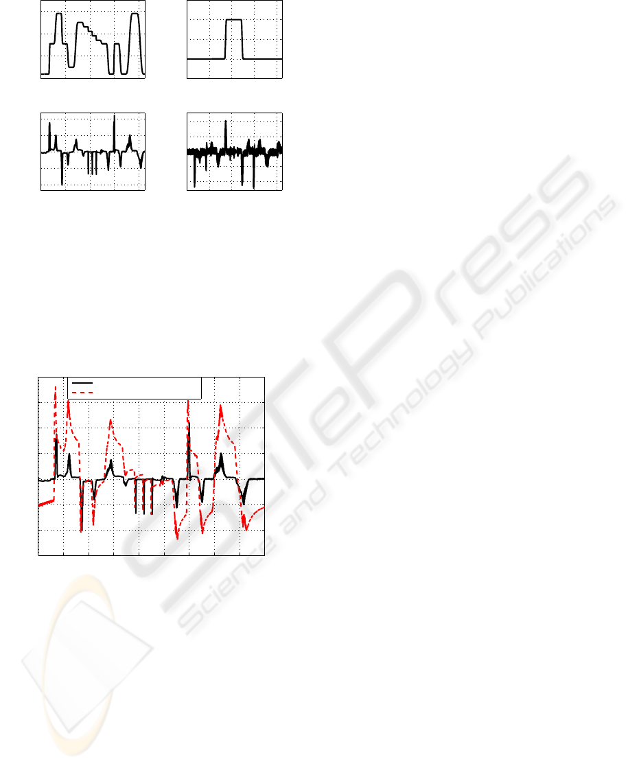
the observer-based disturbance compensation is em-
phasized by Fig. 5. Without this control part the
maximum position control error increases up to ap-
prox. 7 mm.
0 10 20 30 40 50 60 70 80 90
−6
−4
−2
0
2
4
6
8
x 10
−3
t in s
e
x
in m
with disturbance compensation
without disturbance compensation
Figure 5: Position control error e
x
with and without distur-
bance observer (T
P
= 75 ms).
7 CONCLUSIONS
In this paper, a cascaded trajectory control scheme us-
ing nonlinear optimal design is presented for a car-
riage driven by pneumatic muscles. The modelling
of this mechatronic system leads to a system of four
nonlinear differential equations. The nonlinear char-
acteristics of the pneumatic muscles are approximated
by polynomials. The nonlinearity of the valve is lin-
earised by means of a pre-multiplication with its ap-
proximated inverse characteristic. The inner control
loops of the cascade involve a norm-optimal control
of the internal muscle pressure with high bandwidth.
The outer nonlinear model predictive control loop is
responsible for trajectory tracking with carriage po-
sition and mean pressure as controlled variables. Re-
maining model uncertainties are taken into account by
a disturbance force estimated by means of a distur-
bance observer. Experimental results from an imple-
mentation on a test rig emphasise the excellent closed-
loop performance with maximum position errors of
4 mm during the movements, negligible steady-state
position error and steady-state pressure error of less
than 0.02 bar.
REFERENCES
Aschemann, H. and Hofer, E. (2004). Flatness-based tra-
jectory control of a pneumatically driven carriage with
model uncertainties. Proceedings of NOLCOS 2004,
Stuttgart, Germany, pages 239 – 244.
Aschemann, H., Schindele, D., and Hofer, E. (2006). Non-
linear optimal control of a mechatronic system with
pneumatic muscles actuators. CD-ROM-Proceedings
of MMAR 2006, Miedzyzdroje, Poland,.
Carbonell, P., Jiang, Z. P., and Repperger, D. (2001). Com-
parative study of three nonlinear control strategies for
a pneumatic muscle actuator. Proceedings of NOL-
COS 2001, Saint-Petersburg, Russia, pages 167–172.
Fliess, M., Levine, J., Martin, P., and Rouchon, P. (1995).
Flatness and defect of nonlinear systems: Introduc-
tory theory and examples. Int. J. Control 61, 6:1327 –
1361.
Jung, S. and Wen, J. (2004). Nonlinear model predictive
control for the swing-up of a rotary inverted pendu-
lum. ASME J. of Dynamic Systems, Measurement and
Control, 126:666 – 673.
Lizarralde, F., Wen, J., and Hsu, L. (1999). A new model
predictive control strategy for affine nonlinear control
systems. Proc of the American Control Conference
(ACC ’99), San Diego, pages 4263 – 4267.
Lukes, D. (1969). Optimal regulation of nonlinear dynami-
cal systems. SIAM Journal Control, 7:75 – 100.
Weidemann, D., Scherm, N., and Heimann, B. (2004).
Discrete-time control by nonlinear online optimiza-
tion on multiple shrinking horizons for underactuated
manipulators. Proceedings of the 15th CISM-IFToMM
Symposium on Robot Design, Dynamics and Control,
Montreal.
NONLINEAR MODEL PREDICTIVE CONTROL OF A LINEAR AXIS BASED ON PNEUMATIC MUSCLES
99
