INVERSION OF A SEMI-PHYSICAL ODE MODEL
Laurent Bourgois, Gilles Roussel and Mohammed Benjelloun
Laboratoire d’Analyse des Syst
`
emes du Littoral (EA 2600)
Universit
´
e du Littoral - C
ˆ
ote d’Opale
50 rue Ferdinand Buisson, B.P. 699, 62228, Calais Cedex, France
Keywords:
Semi-physical modeling, gray-box, inverse dynamic model, neural network, model fusion.
Abstract:
This study proposes to examine the design methodology and the performances of an inverse dynamic model
by fusion of statistical training and deterministic modeling. We carry out an inverse semi-physical model
using a recurrent neural network and illustrate it on a didactic example. This technique leads to the realization
of a neural network inverse problem solver (NNIPS). In the first step, the network is designed by a discrete
reverse-time state form of the direct model. The performances in terms of generalization, regularization and
training effort are highlighted in comparison with the number of weights needed to estimate the neural network.
Finally, some tests are carried out on a simple second order model, but we suggest the form of a dynamic
system characterized by an ordinary differential equation (ODE) of an unspecified r order.
1 INTRODUCTION
Generally, inverse problems are solved by the in-
version of the direct knowledge-based model. A
knowledge-based model describes system behavior
using the physical, biological, chemical or economic
relationships formulated by the expert. The ”success”
of the data inversion, i.e. the restitution of a nearest
solution in the sense of some ℓ
2
or ℓ
∞
norm distance
from the exact sources of the real system, depends on
the precision of the model, on the noise associated
with the observations and on the method.
Whereas the noise is inherent in the hardware and
conditions of measurement and thus represents a con-
straint of the problem, on the other hand, the two con-
trols an engineer possesses to improve quality of the
estimated solution are the model and the method. The
approach we propose thus relates to these two aspects.
It aims at overcoming several difficulties related to the
definition of the model and its adjustments, and to the
search for a stable solution of the sought inputs of the
system.
2 SEMI-PHYSICAL MODELING
Obtaining a robust knowledge-based model within the
meaning of exhaustiveness compared to the variations
of context (one can also say generic), is often tricky
to express for several reasons. One firstly needs a per-
fect expertise of the field to enumerate all the physical
laws brought into play, all the influential variables on
the system and an excellent command of the subject
to make an exhaustive spatial and temporal descrip-
tion of it. Even if the preceding stage is completed, it
is not rare that some parameters can not be measured
or known with precision. It is then advisable to es-
timate these parameters starting from the observable
data of the system under operation. Once the phys-
ical model has been fixed, it is endowed with good
generics.
A black-box model is a behavior model and de-
pends on the choice of a mathematical a priori form
in which an engineer has a great confidence on its
adaptability with the real behavior of the system. In
the black-box approach, the model precision is thus
dependent on the adopted mathematical form, on the
approximations carried out on the supposed system
order (linear case), on the assumptions of nonlinear-
ity, and on the quantity and the quality of data to make
the identification of the model. Many standard forms
of process (ARMA, ARMAX, NARMAX) (Ljung,
1999) are able to carry out a black-box modeling.
Other techniques containing neural networks have the
characteristic not to specify a mathematical form but
rather a neural structure adapted to the nature of the
system (static, dynamic, linear, nonlinear, exogenic
364
Bourgois L., Roussel G. and Benjelloun M. (2007).
INVERSION OF A SEMI-PHYSICAL ODE MODEL.
In Proceedings of the Fourth International Conference on Informatics in Control, Automation and Robotics, pages 364-371
DOI: 10.5220/0001641803640371
Copyright
c
 SciTePress

input, assumptions on the noise). Neural networks are
known for possessing a great adaptability, with the
properties of universal approximator (Hornik et al.,
1989), (Sontag, 1996) if the available training ex-
amples starting from validated observations are in a
significant number. Nevertheless, black-box models
are less parsimonious than knowledge-based models
since the mathematical functions taking part in the lat-
ter are exact functions (not leaving residues of the out-
put error, without noise). The second disadvantage of
neural black-box models is the least generic behavior
with respect to the new examples which do not form
part of the base of training set. However some tech-
niques exist to improve the generalizing character of
a neural network, like the regularization or the abort
(early stopping) of the training when the error of val-
idation increases.
Between the two types of models previously ex-
posed, (Oussar and Dreyfus, 2001) introduce the
semi-physical or gray-box model. This type of model
fulfills at the same time the requirements of preci-
sion, generics, parsimony of the knowledge-based
models, and also possesses the faculty of training
and adaptability. Close approaches were proposed
by (Cherkassky et al., 2006). These approaches of-
ten consist in doing the emulation of physically-based
process models starting from training of neural net-
works with simulated data (Krasnopolsky and Fox-
Rabinovitz, 2006). If the knowledge model is diffi-
cult to put in equation because of its complexity, the
idea will be to structure a looped neural network (case
of dynamic complex systems) using knowledge on the
fundamental laws which govern the system. Then, we
add degrees of freedom (neurons) to the network to
adapt it to the ignored parts of the system. The recall
phase (production run) then makes it possible to carry
out the predicted outputs in real time.
3 INVERSE NEURAL MODEL
3.1 Principle
The inversion of a physical model generally consists
in estimating information on the nonmeasurable pa-
rameters or inputs starting from the measurable ob-
servations and a priori information on the system. We
propose here to use the training of an inverse model
using a neural network. Some ideas for forward and
inverse model learning in physical remote measure-
ment applications are proposed by (Krasnopolsky and
Schillerb, 2003). It consists in estimating parameters
of the network so that the outputs correspond to the
inputs (or the parameters) desired for training set of
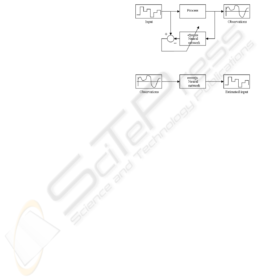
examples (figure 1). In recall phase, the network es-
timates the amplitudes of the parameters or the se-
quence of the input vector for the measured observa-
tions (figure 2), by supposing here that the real model
does not evolve any more after the last training. Here
the model is structured by the inverse model starting
from the direct deterministic model.
Figure 1: Training phase of the inverse neural model.
Figure 2: Recall phase of the inverse neural model.
3.2 Regularization and Inverse Neural
Model
Inverse problems are often ill posed within the mean-
ing of Hadamard (Groetsch, 1993). They can present:
1. An absence of solution;
2. Multiple solutions;
3. An unstable solution.
To transform ill posed problems into well con-
ditioned problems, it is necessary to add a priori
knowledge on the system to be reversed. There
are several approaches which differ by the type of
a priori knowledge introduced (Thikhonov and Ars-
enin, 1977), (Idier, 2001), (Mohammad-Djafari et al.,
2002).
However, can we pose the problem of the regular-
ization in the case of the NNIPS ? In fact, it is clear
that the neural network provides a solution to the pre-
sentation of an input example. Even if this example is
unknown, the network answers in a deterministic way
by a solution, which could be false. From its prop-
erty of classifier and autoassociativity, it will provide
in best case, the most similar solution to the class in-
cluding the test examples. That thus answers difficul-
ties 1 and 2 of the inverse problems, even if the sug-
gested solution can prove to be false. In addition, we
saw above that regularization during training phase,
improves generalization with respect to the examples.
INVERSION OF A SEMI-PHYSICAL ODE MODEL
365

It avoids the problem of overtraining which precisely
results in an instability of the solutions in the vicin-
ity of a point. It is remarkable that the early stopping
method should have an interesting effect on general-
ization and constitute a particular form of the regular-
ization. In other words, we have found, with the neu-
ral networks the techniques usually exploited for the
analytical or numerical inverse problems regulariza-
tion so as to answer risk 3. This confirms our opinion
to use the neural networks like an inverse model.
4 RECURRENT NEURAL
SYSTEMS MODELING
4.1 General Case
In particular, we have been interested in dynamic sys-
tems represented by recurrent equations or finite dif-
ferences. We have chosen to represent the models
by a state space representation because of systems
modeling convenience and for the more parsimonious
character compared to the input-outputs transfer type
models. We have thus made the assumption that
the system can be represented by the following state
equations:

x(n+1) = ϕ[x(n),u(n)]
y(n) = ψ[x(n)]+b(n)
(1)
ϕ is the vector transition function, ψ is the out-
put vector function and b(n) is the output noise to in-
stant n. Under this assumption of output noise, neural
modeling takes the following canonical form (Drey-
fus et al., 2004):

x(n+1) = ϕ
RN
[x(n),u(n)]
y(n) = ψ
RN
[x(n)]+b(n)
(2)
The observation noise appearing only in the ob-
servation equation does not have any influence on the
dynamic of the model. In this case, the ideal model is
the looped model, represented on figure 3.
4.2 Dynamic Semi-Physical Neural
Modeling
The semi-physical model design requires that one
should have a knowledge-based model, usually rep-
resented in the form of an algebraic equation whole,
differential, with partial derivative, sometimes non-
linear coupled. We have examined the modeling of a
system represented by an ordinary differential equa-
tion. To expose the principle, we have again taken
Figure 3: Ideal direct neural model with output noise as-
sumption. The q
−1
operator stands for one T sample time
delay.
the essential phases of semi-physical neural modeling
more largely exposed in (Oussar and Dreyfus, 2001),
(Dreyfus et al., 2004). We have also supposed that
the starting model can be expressed by the continu-
ous state relations:

dx
dt
= f [x(t),u(t)]
y(t) = g[x(t)]
(3)
Where x is the vector of state variables, y is the
output vector, u is the command inputs vector, and
where f and g are vector functions. The functions f
and g can however be partially known or relatively
vague. In a semi-physical neural model, the functions
which are not precisely known are fulfilled by the
neural network, after the preliminary training of the
latter from experimental data. The accurately known
functions are maintained in their analytical form, but
one can also adopt a neural representation whose ac-
tivation function is known and does not use of ad-
justable parameters. The design of a semi-physical
model generally includes four stages:
• Obtaining the discrete knowledge-based model;
• Designing the network in the canonical form (2)
by adding degrees of freedom;
• Initializing from a knowledge-based model simu-
lator;
• Training from the experimental data.
We have applied these steps to an inverse semi-
physical model by adding a stage of inversion of the
discrete model before training.
4.3 An Academic Example: the Direct
Second Order Ode Model
We have studied the deconvolution problem for lin-
ear models governed by an ordinary differential equa-
tion in order to test the method. However, this work
has been only one first step with more general inverse
ICINCO 2007 - International Conference on Informatics in Control, Automation and Robotics
366

problem, which aims, starting from some observa-
tions of the system at carrying out the training of the
inverse model for then being able to estimate the in-
puts and the observable states (within the observabil-
ity sense of the states) of the system. Let us suppose
a system represented by the differential equation:
d
2
y
dt
2
+2ξω
n
dy
dt
+ω
2
n
y = c
1
u(t)
(4)
This second order differential equation could be
the representation of a mechanical system (mass,
spring, shock absorber) or of an electric type (RLC
filter) excited by a time depending input u(t). This
physical model where the kinematic parameters of
damping ξ, natural pulsation ω
n
, and static gain c
1
are
not a priori known, can be represented by the model
of following state:







dx(t)
dt
=
"
0 1
−ω
2
n
1−2ξω
n
#
x(t)+
"
0
c
1
#
u(t)
y(t) =
h
1 0
i
x(t)
(5)
The first stage is supplemented by the discretiza-
tion. By supposing that we have collected the data
with T sampling period, we have proceeded to the dis-
cretization by choosing the explicit Euler method. For
the system (5) to which one has added an observation
noise b(n), the discrete equation of state is obtained:

x(n+1) = Fx(n)+Gu(n)
y(n) = Hx(n)+b(n)
(6)
With:















F =
"
1 T
−ω
2
n
T 1−2ξω
n
T
#
G
T
=
h
0 T
i
H =
h
c
1
0
i
(7)
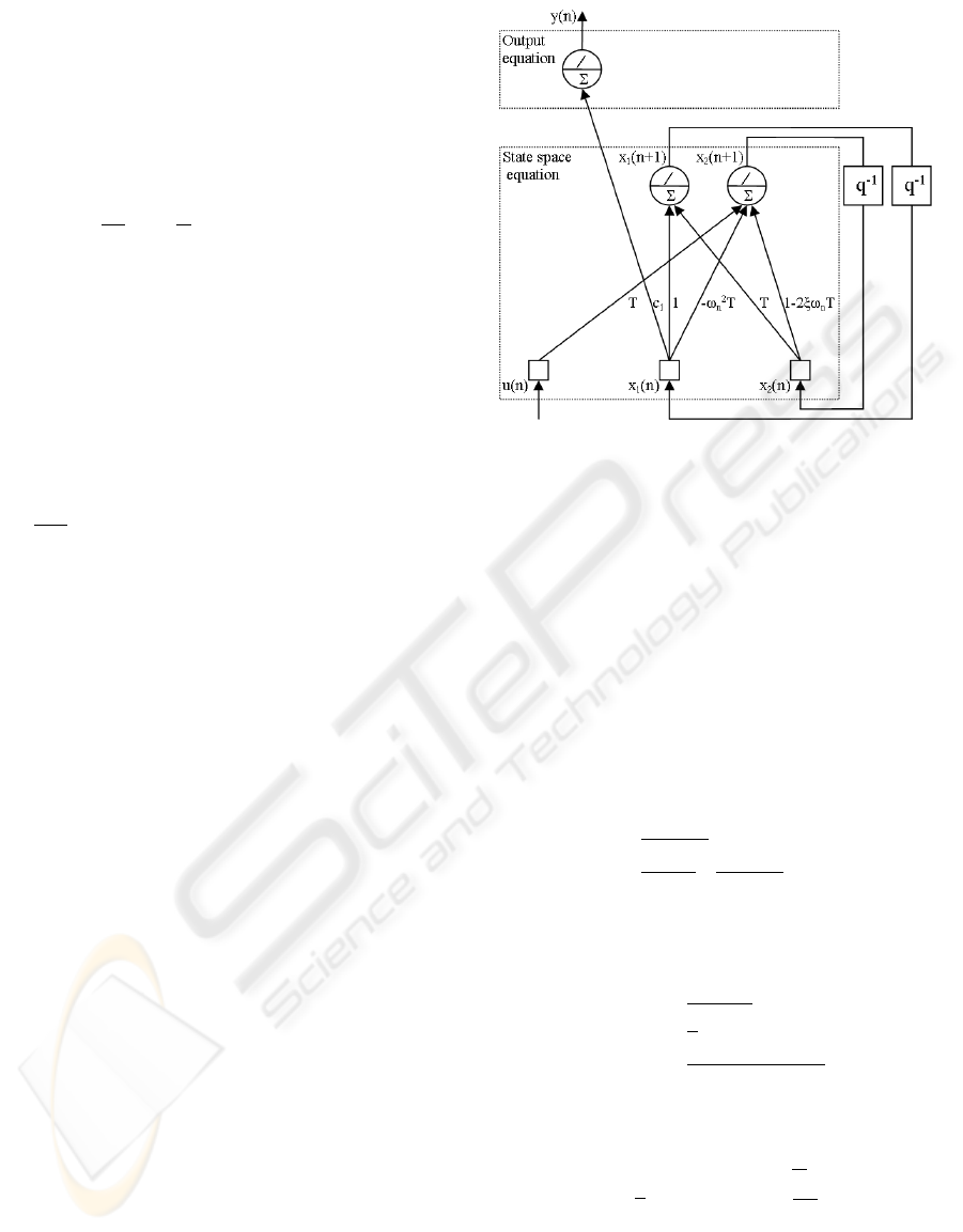
The model in the form of looped neural network of
the nondisturbed canonical system (6), is represented
on figure 4.
The transfer functions represented on figure 4 are
purely linear, being the ideal neural model. No new
degrees of freedom are added to the direct model, this
one being only intermediate representation, nonessen-
tial to the study. It simply illustrates with an example,
the general form of the figure 3.
Figure 4: Direct second order neural model.
5 INVERSE SEMI-PHYSICAL
NEURAL MODEL
5.1 Case of Second Order Model
From the preceding model we have expressed the out-
put u(n) according to the input y(n). The particular
shape of Kronecker of matrices G and H in the re-
lation (6), has enabled us to isolate x
1
(n), x
2
(n) and
u(n):





x
1
(n) =
y(n)−b(n)
c
1
x
2
(n) =
x
1
(n+1)
T
−
y(n)−b(n)
c
1
T
u(n) = αx
1
(n+1)+βx
2
(n+1)+γ[y(n)−b(n)]
(8)
With:





α =
2ξω
n
T−1
T
2
β =
1
T
γ =
(ω
n
T)
2
+(1−2ξω
n
T)
c
1
T
2
(9)
And finally, one has obtained the matrix form:







x(n) =
"
0 0
1
T
0
#
x(n+1)+


1
c
1
−
1
c
1
T


[y(n)−b(n)]
u(n) =
h
α β
i
x(n+1)+γ[y(n)−b(n)]
(10)
Of course, this noncausal equation is realistic only
if we calculate the recurrence by knowing the state at
INVERSION OF A SEMI-PHYSICAL ODE MODEL
367

the moment n + 1 to determine the state at the mo-
ment n. This is more natural to the inverse problem
where we seek to reconstitute the input sequence at
the origin of the generated observations. The equa-
tion now reveals the output noise as a correlated state
noise b(n) and as a noise on the input u(n) with a rate
of amplification equivalent to the real γ. The ideal
looped neural network representation of the model
(10) is given on figure 5. We preserve the delays q
−1
between the states x(n + 1) and x(n) because of the
presentation of the output y(n) and the calculation of
u(n) in reverse-time. In addition, this model remains
stable for any T, the eigenvalues of the reverse-time
state matrix being null for this example.
Figure 5: Inverse second order neural model.
If the sampling period is generally known, coeffi-
cients α, β and γ of the physical model can be impre-
cise, or completely unknown. The degrees of freedom
that can be added to the network can relate to these
parameters, themselves resulting from a combination
of physical parameters. It is then optionally advisable
to supplement this network by adding additional neu-
rons on some internal links where parameters must be
estimated.
5.2 General Case for r Order Ode
without Derivative Input
The general case of the ODE mono input, mono out-
put, continuous, without derivative from the input is
expressed as follows:
a
r
d
r
y
dt
r
+a
r−1
d
r−1
y
dt
r−1
+
· · ·
+a
1
dy
dt
+a
0
y = c
1
u(t)
(11)
In time discretization by sample interval of a low
width T by the Euler’s finite differences method, the
shape of the direct equation matrices F, G and H are
then:

































F =













1 T 0 0
0 1 T
.
.
.
1 T 0
0 0 1 T
−
a
0
T
a
r
· · · −
a
r−1
T
a
r
+1













G
T
=

0 · · · 0 T

H =

c
1
0 · · · 0

(12)
A new system is obtained with the inverse model
expressed in reverse-time:

x(n) = F
I
x(n+1)+G
I
[y(n)−b(n)]
u(n) = H
I
x(n+1)+I
I
[y(n)−b(n)]
(13)
Where the matrices of the inverse state equation
F
I
, G
I
, H
I
and I
I
are all dependent on T. The retro-
grade lower triangular state matrix, of size dim(F
I
) =
r× r and of rank (r− 1), takes the form (14).
F
I
=











0 0
1
T
0
−
1
T
2
1
T
.
.
.
0
−

−
1
T

r−1
−

−
1
T

r−2
· · ·
1
T
0











(14)
The output application matrix G
I
, of dimension
dim(G
I
) = r× 1 becomes (15).
G
T
I
=

1
c
1
−
1
c
1
T
1
c
1
T
2
· · ·
1
c
1

−
1
T

r−1

(15)
The input matrix of dimension dim(H
I
) = 1× r is
worth (16).
H
I
=
h
0 · · · 0
1
T
i
+

a
0
a
r
· · ·
a
r−2
a
r
−
1
T

1−
a
r−1
T
a
r
 
F
I
(16)
The direct application matrix I
I
of the output to the
input, of dimension dim(I
I
) = 1× 1 is given by (17).
ICINCO 2007 - International Conference on Informatics in Control, Automation and Robotics
368

I
I
=

a
0
a
r
· · ·
a
r−2
a
r
−
1
T

1−
a
r−1
T
a
r
 
G
I
(17)
If it is considered that the representation of the in-
verse model (1) takes the form (18), the general neu-
ral representation of the inverse model takes the form
shown on figure 6.

x(n) = ϕ
I
RN
[x(n+1),y(n)]
u(n) = ψ
I
RN
[x(n+1),y(n)]
(18)
In Which ϕ
I
RN
(F
I
,G
I
) is related to transition to
reverse-time and Ψ
I
RN
(H
I
,I
I
) represents the restoring
function of the input. On the numerical level, the
eigenvalues of the matrix F
I
in ODE case being all
null, thus there is no risk of instability.
Figure 6: Neural representation of the reverse state model.
6 RESULTS
The goal of this section is to check the assumptions
of awaited quality concerning the two NNIPS (black-
box and gray-box models) in terms:
• of robustness with respect to an unknown input
from the base of training compared to the inverse
state model;
• of robustness with respect to the noise on the out-
put (i.e. the regularizing effect) compared to the
inverse state model;
• of gain in effort of training.
The black-box neural model is an Elman network
with two linear neurons on its hidden layer, and with
one neuron on its output layer. This neural network
is fully connected, and the weights and biases are
initialized with the Nguyen-Widrow layer initializa-
tion method (Nguyen and Widrow, 1990). The semi-
physical model design is carried out from the preced-
ing black-box model which has been modified to ob-
tain the neural representation of the figure 5. For that,
the coefficients depending on the parameters T, c
1
,
α, β and γ are left free. Only three coefficients have
been forced to be null to delete corresponding con-
nections. We have also connected the inputs layer to
the output layer, but we have not added any additional
neuron. These two models are subjected to a training
with (pseudo) experimental disturbed data. For the
numerical tests, we have adopted the parameters ac-
cording to ω
n
= 5 rad.s
−1
, ξ = 0.4, T = 0.05 s and
c
1
= 1. It is noticed that this choice of parameters en-
sures, for the matrix F of the system (6), a spectral
radius lower than 1, and consequently the stability of
the direct model.
To construct the sets of training, we have gener-
ated a N samples input random sequence to simulate
the direct knowledge-based model. This signal is a
stochastic staircase function, resulting from the prod-
uct of an amplitude level A
e
by a Gaussian law of
average µ
e
and variance σ
2
e
, of which the period of
change T
e
of each state is adjustable. T
e
influences the
input signal dynamics, and thus the spectrum of the
system excitation random signal. For all the tests, we
have fixed A
e
= 1, µ
e
= 0, σ
2
e
= 1, T
e
= 60T, T
b
= 3T
and µ
b
= 0. This input signal provides a disturbed
synthetic output signal. The variance σ
2
b
, the average
µ
b
, as well as the period of change of state T
b
charac-
terize the dynamics of the noise.
Weights Initial Value: The stage of coefficients ini-
tialization being deterministic for the quality of the
results in the black-box model case, we have cho-
sen to reproduce hundred times each following exper-
iments. Indeed, some initial values can sometimes
generate mean squared error (MSE) toward infinite
value. These results will then be excluded before car-
rying out performances and average training efforts
calculation.
6.1 Test On Modeling Errors and
Regularizing Effect
We have measured the generalization and regulariza-
tion contribution of the inverse neural model com-
pared to the inverse state model. For that, we have
compared the mean square errors of the inverse state
model with those obtained in phase of recall of the
two inverse neural form models.
6.1.1 Training and Test Signals and Comparison
of Restorations
We have tested five training sequences length N = 300
samples. The variances which characterize the dy-
namics of the noise in the pseudo experimental sig-
nals σ
2
b
are worth 0, 0.03, 0.09, 0.25, and 1. They
generate for the process output signal several values
of signal to noise ratio (SNR) from around 20 dB to
infinity. Then we have compared the MSE of decon-
volution in recall phase with new disturbed random
INVERSION OF A SEMI-PHYSICAL ODE MODEL
369

signals with the same variances and applied to the in-
verse black-box and semi-physical models.
6.1.2 Numerical Results
Let us underline the fact that only seventy-six experi-
ments have been retained for calculation of averages.
The black-box model have not provided (due to a bad
initialization of the coefficients) suitable restoration
in 24% of the cases. The figure 7 gathers the results
of MSE for the three inverse models. The figure 8
illustrates the signals obtained for the output signals
deconvolutions with a SNR of 33 dB.
19 33 44 55 Inf
0
0.2
0.4
0.6
0.8
1
1.2
1.4
1.6
1.8
2
SNR in dB of signal to reverse
Mean squared error
Comparison of performances of regularization for differents SNR values
Inverse state model
Black−box neural network
Semi−physical neural network
Figure 7: Impact of neural models on the regularization:
evolution of the three models MSE according to the SNR.
0 50 100 150 200 250 300
−5
0
5
10
Time
Signals
Input and output signals
0 50 100 150 200 250 300
−10
0
10
20
Time
Signals
Comparison between the test input and the estimated input (inverse state model)
0 50 100 150 200 250 300
−5
0
5
10
Time
Signals
Comparison between the test input and the estimated input (inverse models)
Test input
Estimated input (black−box neural network)
Estimated input (semi−physical neural network)
Test input
Estimated input (inverse state model)
Test input
Second−order output (without noise)
Second−order output (with noise)
Figure 8: a) Test signals (SNR of 33 dB), b) Deconvolution
by the reverse state model, c) Deconvolution by the inverse
neural models.
Noiseless case: In absence of noise in training and
test signals, black-box and semi-physical models pro-
vide similar mean performances (MSE of approxi-
mately 0.18) and in addition relatively near to the in-
verse state model.
Noisy case: When the noise grows in the training and
test signals, the two neural models are much less sen-
sitive to the noise than the inverse state model (figure
7). The regularizing effect is real. The semi-physical
model has good performances but, the constraint im-
posed by the structure of the network and the more
reduced number of connections (synapses), decreases
the robust effect to the noise (loss of the neural net-
work associative properties) and slightly places this
model in lower part of the black-box model. It is
thus noted that performances in term of regulariza-
tion are much better than for the inverse state model,
but a little worse than for the black-box model (MSE
increases more quickly). The performances seem to
be a compromise between the knowledge-based and
the black-box model. Let us note that this difference
grows with a higher order model and also increases
the number of neurons.
6.2 Test On Learning Effort
For this test, we have compared the product of the
MSE by the number of epochs, i.e. the final error
amplified by the iteration count of the training phase.
Learning stops if the iteration count exceeds 250 or if
MSE is lower than 0, 03. We have made a distinction
between errors at the end of the training (figure 9) and
errors on the test as a whole (figure 10).
19 33 44 55 Inf
10
15
20
25
30
35
40
SNR in dB of signal to reverse
MSE
1
*epochs
Comparison of the training efforts for differents SNR values
Black−box neural network
Semi−physical neural network
Figure 9: Curves of learning effort on the training set.
As learning effort depends on the number of neu-
rons, one compares the black-box and gray-box net-
works with an equal number of neurons. In the first,
all the weights of connections are unknown. In the
second, one considers all the weights with the excep-
tion of the three coefficients corresponding to non-
existent connections and being null. On figure 9, we
note that the gray-box model is more effective when
the noise is weak. Physical knowledge supports the
convergence of the weights so that the behavior ap-
proaches the data. This seems to be checked un-
til SNR of about 20 dB as in our example. Beyond
ICINCO 2007 - International Conference on Informatics in Control, Automation and Robotics
370

19 33 44 55 Inf
30
35
40
45
50
55
60
65
70
SNR in dB of signal to reverse
MSE
2
*epochs
Comparison of the training efforts for differents SNR values
Black−box neural network
Semi−physical neural network
Figure 10: Curves of learning effort on the test set.
that, it is the black-box which is slightly more effec-
tive. On figure 10, the tendencies are the same for the
black-box model. The gray-box model is penalized
by the constraint imposed by the neural framework
and the more reduced number of connections. Within
the framework of a traditional second order ODE, the
semi-physical model seems to require a greater effort
with the test set than the black-box model. Indeed,
within the framework of this example, the number of
coefficients remaining free for the gray-box model be-
ing relatively low, it leads to a loss of the generaliza-
tion capacity compared to the black-box model. How-
ever, this supremacy is quite relative since only 76%
of the tests carried out have been conclusive for the
black-box model and 100% for the gray-box model.
7 CONCLUSION
We have examined the performances of an inverse dy-
namic model by fusion of statistical learning and de-
terministic modeling. For the study, our choices have
gone toward the design of an inverse semi-physical
model using a looped neural network. We have com-
pared the latter with an inverse fully connected neu-
ral network. Experimental results on a second order
system have shown that the inverse gray-box neural
model is more parsimonious and presents better per-
formances in term of learning effort than the inverse
black-box neural model, because of knowledge in-
duced by the deterministic model. The performances
in term of inverse modeling precisions are visible
since the input restoration errors are weak. The neu-
ral training plays the part of statistical regressor and of
regularization operator. Finally, a higher order model
increases the number of neurons and then improves
the robust effect to the noise of the gay-box model.
REFERENCES
Cherkassky, V., Krasnopolsky, V. M., Solomatine, D., and
Valdes, J. (2006). Computational intelligence in earth
sciences and environmental applications: Issues and
challenges. Neural Networks, 19, issue 2:113–121.
Dreyfus, G., Martinez, J. M., Samuelides, M., Gordon,
M. B., Badran, F., Thiria, S., and H
´
erault, L. (2004).
R
´
eseaux de Neurones: M
´
ethodologies et Applications.
Eyrolles, 2
`
eme
´
edition, Paris.
Groetsch, C. W. (1993). Inverse Problems in the Mathemat-
ical Sciences. Vieweg Sohn, Wiesbaden.
Hornik, K., Stinchcombe, M., and White, H. (1989). Multi-
layer feedforward networks are universal approxima-
tors. Neural Networks, 2:359–366.
Idier, J. (2001). Approche Bayesienne pour les Probl
`
emes
Inverses. Trait
´
e IC2, S
´
erie Traitement du Signal et de
l’Image, Herm
`
es, Paris.
Krasnopolsky, V. M. and Fox-Rabinovitz, S. F. (2006).
Complex hybrid models combining deterministic and
machine learning components for numerical climate
modeling and weather prediction. Neural Networks,
19:122–134.
Krasnopolsky, V. M. and Schillerb, H. (2003). Some neural
network applications in environmental sciences. part i:
Forward and inverse problems in geophysical remote
measurements. Neural Networks, 16:321–334.
Ljung, L. (1999). System Identification, Theory for the
User. Prentice Hall, N. J.
Mohammad-Djafari, A., Giovannelli, J. F., Demoment, G.,
and Idier, J. (2002). Regularization, maximum en-
tropy and probabilistic methods in mass spectrometry
data processing problems. Int. Journal of Mass Spec-
trometry, 215, issue 1:175–193.
Nguyen, D. and Widrow, B. (1990). Improving the learning
speed of 2-layer neural networks by choosing initial
values of the adaptive weigths. Proceedings of the
International Joint Conference on Neural Networks,
3:21–26.
Oussar, Y. and Dreyfus, G. (2001). How to be a gray box
: Dynamic semi-physical modeling. Neurocomputing,
14:1161–1172.
Sontag, E. D. (1996). Recurrent neural networks : Some
systems-theoretic aspects. Technical Report NB, Dept
of mathematics, Rutgers University, U.S.A.
Thikhonov, A. N. and Arsenin, V. Y. (1977). Solutions of ill
Posed Problems. John Wiley, New York.
INVERSION OF A SEMI-PHYSICAL ODE MODEL
371