TRANSFORMATION ANALYSIS METHODS
FOR THE BDSPN MODEL
Karim Labadi
EPMI- ECS, 13 boulevard de l’Hautil 95092 Cergy Pontoise Cedex, France
Haoxun Chen and Lionel Amodeo
LOSI-ICD (FRE CNRS 2848), 12 rue Marie Curie, BP 2060, 10010 Troyes Cedex, France
Keywords: Petri nets, BDSPN model, modelling, analysis, discrete event systems.
Abstract: The work of this paper contributes to the structural analysis of batch deterministic and stochastic Petri nets
(BDSPNs). The BDSPN model is a class of Petri nets introduced for the modelling, analysis and
performance evaluation of discrete event systems with batch behaviours. The model is particularly suitable
for the modelling of flow evolution in discrete quantities (batches of variable sizes) in a system with
activities performed in batch modes. In this paper, transformation procedures for some subclasses of
BDSPN are developed and the necessity of the introduction of the new model is demonstrated.
1 INTRODUCTION
A Petri net model, called batch deterministic and
stochastic Petri nets (BDSPN), was introduced for
the modelling, and performance evaluation of
discrete event systems with batch behaviours. As we
know, industrial systems are often characterized as
batch processes where materials are processed in
batches and many operations are usually performed
in batch modes to take advantages of the economies
of scale or because of the batch nature of customer
orders. It is shown in our previous papers that the
model is a powerful tool for both analysis and
simulation of those systems and its capability to
meet real needs was demonstrated through
applications to logistical systems (Labadi, et al.
2005, 2007; Chen, et al. 2005). The objective of this
paper is to study the transformation of a BDSPN
model into an equivalent classical Petri net model.
Such a transformation is possible for some cases for
which the corresponding transformation procedures
are developed. We will also show that for the model
with variable arc weights depending on its marking,
the transformation is impossible. This study allows
us to establish a relationship between BDSPNs and
classical discrete Petri nets and to demonstrate the
necessity of introducing the BDSPN model.
2 DESCRIPTION OF THE
MODEL
BDSPN model is developed from deterministic and
stochastic Petri nets (Marsan, et al. 1987;
Lindemann, 1998) by introducing batch components
(batch places, batch tokens, and batch transitions)
and new transition enabling and firing rules. Firstly,
we recall the basic definition and the dynamical
behavior of the model (Labadi, et al. 2005, 2007;
Chen, et al. 2005).
2.1 Definition of the Model
A BDSPN is a nine tuple (P, T, I, O, V, W, Π, D, µ
0
)
where:
P = P
d
∪ P
b
is a finite set of places consisting of
the discrete places in set P
d
and the batch places in
set P
b
. Discrete places and batch places are
represented by single circles and squares with an
embedded circle, respectively. Each token in a
discrete place is represented by a dot, whereas each
batch token in a batch place is represented by an
Arabic number that indicates its size.
T = T
i
∪ T
d
∪ T
e
is a set of transitions consisting
of immediate transitions in set T
i
, the deterministic
timed transitions in set T
d
, and exponentially
distributed transitions in set T
e
. T can also be
135
Labadi K., Chen H. and Amodeo L. (2007).
TRANSFORMATION ANALYSIS METHODS FOR THE BDSPN MODEL.
In Proceedings of the Fourth International Conference on Informatics in Control, Automation and Robotics, pages 135-141
DOI: 10.5220/0001638501350141
Copyright
c
 SciTePress

partitioned into T
D
∪ T
B
: a set of discrete transitions
T
D
and a set of batch transitions T
B
. A transition is
said to be a batch transition (respectively a discrete
transition) if it has at least an input batch place
(respectively if it has no input batch place).
I ⊆ (P × T), O ⊆ (T × P), and V ⊆ (P × T) define
the input arcs, the output arcs and the inhibitor arcs
of all transitions, respectively. It is assumed that
only immediate transitions are associated with
inhibitor arcs and that the inhibitor arcs and the input
arcs are two disjoint sets.
W: (I ∪ O ∪ V)×IN
|P|
→IN, where IN is the set of
nonnegative integers, defines the weights for all
ordinary arcs and inhibitor arcs. For any arc (i, j) ∈
I ∪ O ∪ V, its weight W(i, j) is a linear function of
the M-marking with integer coefficients
α , β , i.e.,
w(i, j) = α
ij
+ ∑
p∈ P
β
(i, j)p
× M(p). The weight w(i, j)
is assumed to take a positive value.
Π: T→IN is a priority function assigning a
priority to each transition. Timed transitions are
assumed to have the lowest priority, i.e.; Π(t) = 0 if t
∈ T
d
∪ T
e
. For each immediate transition t ∈ T
i
,
Π(t) ≥ 1.
D: T→[0, ∞) defines the firing times of all
transitions. It specifies the mean firing delay for
each exponential transition, a constant firing delay
for each deterministic transition, and a zero firing
delay for each immediate transition
µ
0
: P→IN ∪ 2
IN
is the initial µ-marking of the
net, where 2
IN
consists of all subsets of IN, µ
0
(p) ∈
IN if p ∈ P
d
, and µ
0
(p) ∈ 2
IN
if p ∈ P
b
.
The state of the net is represented by its µ-
marking. We use two different ways to represent the
µ-marking of a discrete place and the µ-marking of a
batch place. The first marking is represented by a
nonnegative integer, whereas the second marking is
represented by a multiset of nonnegative positive
integers. The multiset may contain identical
elements and each integer in the multiset represents
a batch token with a given size. Moreover, for
defining the net, another type of marking, called M-
marking, is also introduced. For each discrete place,
its M-marking is the same as its μ-marking, whereas
for each batch place its M-marking is defined as the
total size of the batch tokens in the place.
2.2 Transition Enabling and Firing
The state or µ-marking of the net is changed with
two types of transition firing called “batch firing”
and “discrete firing”. They depend on whether a
transition has no batch input places. In the
following, a place connected with a transition by an
arc is referred to as input, output, and inhibitor
place, depending on the type of the arc. The set of
input places, the set of output places and the set of
inhibitor places of transition t are denoted by
•
t, t
•
,
and
° t, respectively, where
•
t = { p | (p, t) ∈ I }, t
•
=
{ p | (t, p) ∈ O }, and
° t = { p | (p, t) ∈ V }. The
weights of the input arc from a place p to a transition
t, of the output arc from t to p are denoted by w(p, t),
w(t, p) respectively.
2.2.1 Batch Enabling and Firing Rules
A batch transition t is said to be enabled at µ-
marking µ if and only if there is a batch firing index
(positive integer) q∈IN (q > 0) such that:
() ( )
,: ,
b
ptPbμ pqbwpt
•
∀∈ ∩ ∃∈ = (1)
() ( )
, ,
d
ptP Mpqwpt
•
∀∈ ∩ ≥×
(2)
() ( )
, ,pt Mpwpt∀∈ <
D
(3)
The batch firing of t leads to a new µ-marking µ’:
() () ( )
:' ,
d
ptPμ p μ pqwpt
•
∀∈ ∩ = −×
(4)
() () ( )
{}
:' ,
b
ptPμ p μ pqwpt
•
∀∈ ∩ = − × (5)
() () ( )
:' ,
d
pt Pμ p μ pqwtp
•
∀∈ ∩ = +×
(6)
() () ( )
{}
•
:' ,
b
pt Pμ p μ pqwtp∀∈ ∩ = + ×
(7)
2.2.2 Discrete Enabling and Firing Rules
A discrete transition t is said to be enabled at µ-
marking µ (its corresponding M-marking M) if and
only if:
() ( )
, ,pt Mpwpt
•
∀∈ ≥
(8)
() ( )
, ,pt Mpwpt∀∈ <
D
(9)
The discrete firing of t leads to a new µ-marking µ’:
() () ( )
•
∀∈ = −: ' ,pt μ p μ pwpt
(10)
() () ( )
•
∀∈ ∩ = +: ' ,
d
pt P μ p μ pwtp
(11)
() () ( )
{}
•
∀∈ ∩ = +: ' ,
b
pt P μ p μ pwtp
(12)
2.2.3 An Illustrative Example
We describe as an example the BDSPN model of a
simple assembly-to-order system that requires two
components shown in Fig. 1. In the model, discrete
places p
1
and p
2
are used to represent the stock of
component A and the stock of component B
respectively. Batch place p
3
is used to represent
batch customer orders with different and variable
sizes. To fill a customer order of size b, we need b
×
w(p
1
, t
1
) = 2b units of component A from the stock
ICINCO 2007 - International Conference on Informatics in Control, Automation and Robotics
136

represented by p
1
and b × w(p
2
, t
1
) = b units of
component B from the stock represented by p
2
.
These components will be assembled to b units of
final product to fill the order. For instance, at the
current µ-marking µ
0
= (4, 3, {4, 2, 3}, ∅ , 0)
T
, it is
possible to fill the batch customer order b = 2 in
batch place p
3
since the batch transition t
1
is enabled
with q = b/ w(p
3
, t
1
) = 2. After the batch firing of
transition t
1
(start assembly), the corresponding
batch token b = 2 will be removed from batch place
p
3
, q × w(p
1
, t
1
) = 4 discrete tokens will be removed
from discrete place p
1
, and q × w(p
2
, t
1
) = 2 discrete
tokens will be removed from discrete place p
2
. A
batch token with size equal to q
× w(t
1
, p
4
) = 2 will
be created in batch place p
4
and 2 discrete tokens
will be created in discrete place p
5
. Therefore, the
new µ-marking of the net after the batch firing is: µ
1
= (0, 1, {4, 3}, {2}, 2)
T
and its corresponding M-
marking is M
1
= (0, 1, 7, 2, 2)
T
.
t1
p1
p2
2
Batch assembly
operation
p4
4
p3
t2
2
Arrival of batch
customer orders
Replenishment of
component B
Replenishment of
component A
3
p5
Stock 1
Stock 2
Outstanding
b
atch orders
Start
assembly
End
assembly
Figure 1: An assembly-to-order system.
2.3 Reachability Graph
For the analysis of the transformation procedures
developed in the rest of this paper, we need to define
in the following the concept of the reachability
graph of the model.
A µ-marking reachability graph of a given
BDSPN is a directed graph (V
μ
, E
μ
), where the set of
vertices V
μ
is given by the reachability set (µ
0
*
: all
μ-markings reachable from the initial marking
μ
0
by
firing a sequence of transitions and the initial
marking), while the set of directed arcs E
μ
is given
by the feasible µ-marking changes in the BDSPN
due to transition firing in all reachable μ-markings.
Similarly, we define M-marking reachability
graph (V
M
, E
M
) which can be obtained from (V
μ
, E
μ
)
by transforming each μ-marking in V
μ
into its
corresponding M-marking and by merging
duplicated M-markings (and duplicated arcs).
3 TRANSFORMATION
METHODS
The objective of this section is to study the
transformation of a BDSPN model into an
equivalent classical Petri net model.
3.1 Special Case
Firstly, we consider the case where all batch tokens
in each batch place of the BDSPN are always
identical. A batch place p
i
is said to be simple if the
sizes of its all batch tokens are the same for any µ-
marking reachable from µ
0
.
2
p
1
p
2
3
2
p
3
6
6
6
t1
36
0
2
12
9
8
6
18
14
0
31
20
t1 t1 t1
M-marking graph
T
ransformat
i
on
{6, 6, 6}
∅
2
{6, 6}
{9}
8
{6}
{9, 9}
14
t1
[3]
t1
[3]
t1
[3]
∅
{9, 9,9}
20
(
a
)
(6/2)×2
p
1
p
2
(6/2)×3
(6/2)×2
p
3
t1
(
b
)
Figure 2: Transformation of a BDSPN (special case).
To illustrate the transformation method, we consider
an example given in Fig. 2. The net (a) whose all
batch places are simple can be easily transformed
into an equivalent classical discrete Petri net (b). We
observe that the two nets have the same M-marking
reachability graph (the same dynamical behaviour).
Indeed, the two properties, (i) all batch places of the
net are simple and (ii) the net has no variable arc
weight, lead to a constant batch firing index q
j
for
each batch transition t
j
∈ T
b
of the net. As
formulated in the following procedure, the
transformation method consists of (i) transforming
each batch place into a discrete place and (ii)
integrating the constant batch firing index of each
batch transition in the weights of its input and output
arcs in the resulting classical net in order to respect
TRANSFORMATION ANALYSIS METHODS FOR THE BDSPN MODEL
137

the dynamic behaviour of the original batch net.
Transformation procedure (special case)
Given a BDSPN whose all batch places are simple
and whose all arcs have a constant weight. This net
can be transformed into an equivalent classical
discrete Petri net, denoted by DPN by the following
procedure:
Step1
. The set of discrete places P
d
of the BDSPN
and their markings remain unchanged for the DPN.
00
, () ()
id i i
pPMp μ p∀∈ =
(13)
Step2. Each batch place of the BDSPN is
transformed into a discrete place M-marked in the
DPN.
(
)
()
∈
∀∈ =
∑
0
,
i
ib i
b μ p
pPMp b
(14)
Step3
. The set of transitions T of the BDSPN
remains unchanged for the DPN.
Step4. The weight of each output arc of each batch
place p
i
∈ P
b
of the BDSPN is set to the size of its
batch tokens b
i
.
•
∗
∀∈ ∀∈
=× =
, ,
(,) (,)
(,)
ibji
i
ij ij i
ij
pPt p
b
Wpt Wpt b
Wp t
(15)
Step5
. The weight of each output arc of each batch
transition t
j
∈ T
b
of the BDSPN is set to its original
weight multiplied by its batch firing index q
j
.
•∗
∀∈ ∀∈
=×=×
, , ( , )
(, ) (, ) .
(,)
ibji ji
i
ji j ji
ij
pPt pWtp
b
Wt p q Wt p
Wp t
(16)
Step6
. The weight of each output arc of each
discrete transition t
j
∈ T
d
of the BDSPN remains
unchanged for the DPN.
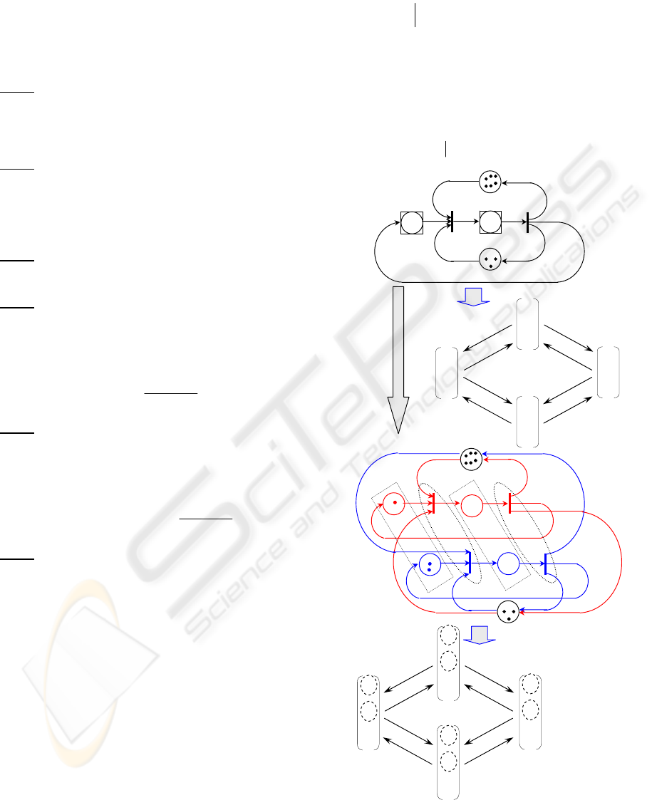
3.2 General Case
The proposed transformation procedure can be
generalized to allow the transformation of a BDSPN
containing batch places which are not simple into an
equivalent classical Petri net. The transformation is
feasible if we know in advance all possible batch
firings of all batch transitions and all possible batch
tokens which can appear in each batch place of the
net during its evolution. In other words, the
transformation can be performed when we well
know the dynamic behaviour of the BDSPN for its
given initial µ-markings µ
0
.
(a) Let D(t
j
) denote the set of all q-indexed
transitions t
j[q]
generated by the firings of the batch
transition t
j
with all possible batch firing indexes q
during the evolution of the BDSPN starting from µ
0
.
[] []
=∃∈ →
*
0
() { ,[ }
j
jq jq
Dt t μμμt
(17)
where µ
0
denotes the set of reachable µ-markings
from µ
0
and µ[t
j[q]
→ denote that the batch transition
t
j
can be fired from µ with a batch firing index q.
(b) Let D(p
i
) denote the set of all possible batch
tokens which can appear in the batch place p
i
during
the evolution the BDSPN starting from µ
0
.
=∃∈ ∈
*
0
() { , ()}
ii
Dp b μμb μ p
(18)
p1
p2
t1
t2
p4
p3
2
2
1
2
(a)
p4
2
2
p3
p2
[2]
t2
[1]
p1[2]
t1
[2]
p1[1] t1
[1]
t2
[1]
p2
[1]
4
4
2
2
2
1
1
2
2
2
(b)
µ
0
µ
1
µ
2
µ
3
t1
[1]
t2
[1]
t2
[2]
t2
[1]
t1
[2]
t1
[1]
t2
[2]
t1
[2]
{1, 2}
∅
6
3
{1}
{2}
2
1
∅
{1, 2}
0
0
{2}
{1}
4
2
Reachability graph of the net (a)
t1
[1]
t2
[1]
t2
[2]
t2
[1]
t1
[2]
t1
[1]
t2
[2]
t1
[2]
1
2
0
0
6
3
1
0
0
2
2
1
0
0
1
2
0
0
0
2
1
0
4
2
M
0
M
1
M
2
M
3
Reachability graph of the net (b)
Figure 3: Transformation of a BDSPN (general case).
By analogy with the transformation procedure
ICINCO 2007 - International Conference on Informatics in Control, Automation and Robotics
138

for the special case, the transformation for the
general case consists of the transformation of its
each batch place p
i
into a set of discrete places
corresponding to D(p
i
) and the transformation of its
each batch transition t
j
into a set of discrete
transitions corresponding to D(t
j
). For example, the
transformation of the BDSPN given in Fig. 3 is
realized by transforming the batch transition t
1
(resp.
t
2
) into a set of discrete transitions {t
1[1]
, t
1[2]
} (resp
{t
2[1]
, t
2[2]
}) and by transforming the batch place p
1
(resp. p
2
) into a set of discrete places {p
1[1]
,p
1[2]
}
(resp. {p
2[1]
, p
2[2]
} as shown in Fig. 3b. Similar to the
special case, to respect the dynamical behaviour of
the BDSPN, each possible batch firing index of each
batch transition is integrated in the weights of the
input and output arcs of the corresponding transition
in the resulting classical net. After a close look of
the reachability graphs of the two nets, we find that
the two nets have the same behaviour. As illustrated
in the figure, each µ-marking µ
i
of the BDSPN
corresponds to the marking M
i
of the resulting
classical Petri net. The M-marking of each batch
place p
i
is expressed by its corresponding set of
discrete places D(p
i
). The transformation procedure
for the general case is outlined in the following.
Transformation procedure (general case)
Step1
. The set of discrete places P
d
of the BDSPN
and their markings remain unchanged for the DPN.
00
, () ()
id i i
pPMp μ p∈=
(19)
Step2
. Each batch place p
i
of the BDSPN is
converted into a set of discrete places D(p
i
) in the
DPN such as:
[]
[] []
()
()
∈=
=∈
∀∈ =
∑
0
and
( ) { ( )} and
(),
i
ii
ib
i
ib ib
l μ plb
Dp p b Dp
pDpMp l
(20)
Step3
. Each batch transition t
j
of the BDSPN is
converted into a set of discrete transitions D(t
j
) in the
DPN such that:
[] []
=∈() { ()}
jj
jq jq
Dt t t Dt
(21)
The set of discrete transitions T
b
of the BDSPN
remains unchanged for the DPN.
Step4
. Each place
[]
()
i
ib
pDp∈
is connected to the
output transitions
[]
•
()
ib
p
such that:
[] []
[]
•
∀∈
=∈ =
•
(),( )
{ and / ( , )}.
i
ib ib
ji ij
jq
pDpp
ttp qbWpt
(22)
[] [] []
[] []
•
∀∈ ∀∈
=×
(), ( )
(,) (,).
ii
bjqib
ij
ib jq
pDpt p
Wp t Wp t b
(23)
Step5
. Each transition
[]
()
j
jq
tDt∈
is connected to
the output places
[]
()
jq
t
•
such that:
[] []
[] []
•
•
•
∀∈ =
∈∈∩
=
∪∈∩
(),( )
{( ()),( )
and ( / ( , ))}
{}.
j
jq jq
iijd
ib ib
ij
ii j d
tDtt
pp Dp ptP
qbWpt
pp t P
(24)
The weights of the corresponding arcs are given by:
[] [] []
[] []
•
∀∈ ∀∨ ∈
=×
(),( ) ( ),
(, ) (,).
ji
jq ib jq
ji
jq ib
tDtpp t
Wt p q Wt p
(25)
Step6
. Each place
[]
()
i
ib
pDp∈
is connected to the
input transitions
[]
()
ib
p
•
such that:
[] []
[]
•
∀∈ =
∈=
∪∈ ∩
•
•
(), ( )
{ and /(,)}
{( )}.
i
ib ib
j
iji
jq
jid
pDp p
tt p qbWtp
tpP
(26)
The weights of the corresponding arcs are given by:
[] [] []
[] []
•
∀∈ ∀∨ ∈
=×
(), ( ) ( )
(, ) (,).
iij
bjqib
ji
jq ib
pDp tt p
Wt p q Wt p
(27)
Step7
. Each transition
[]
()
j
jq
tDt∈
will be
connected to the set
[]
()
j
q
t
•
of input places such that:
[] []
[]
•
•
•
∀∈ =
∈∩ =
∪∈∩
(),( )
{ ( ) and ( / ( , ))}
{}.
j
jq jq
ijd ij
ib
ii j d
tDtt
pptP qbWpt
pp t P
(28)
The weights of the corresponding arcs are given by:
[] [] []
[] [] []
•
∀∈ ∀∨ ∈
=×
(),( ) ( ),
(,) (,).
ji
jq ib jq
i
ib jq jq
tDtpp t
Wp t q Wp t
(29)
Step8. The arcs which connect discrete places with
discrete transitions in the BDSPN and their weights
remain unchanged in the DPN.
3.3 Case with Inhibitor Arcs
The transformation is also possible for BDSPNs
with inhibitor arcs whose weights are constant. We
will illustrate it by using some examples.
Sub-case 1.
As shown in the net depicted in Fig.
4a, in the case where there is an inhibitor arc
connecting a discrete place p
i
to a batch transition t
j
,
the corresponding inhibitor condition must be
TRANSFORMATION ANALYSIS METHODS FOR THE BDSPN MODEL
139

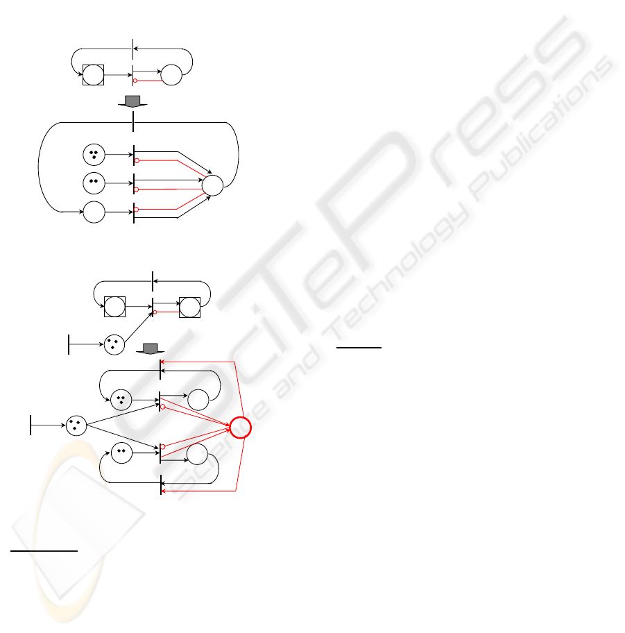
reproduced in the resulting classical Petri net for all
q-indexed transitions t
j[q]
generated by the batch
transition t
j
. Clearly, in this example, the batch
transition t
1
can be fired with three possible batch
firing indexes during the evolution of the net. In
other words, the transition t
1
generates three possible
q-indexed transitions t
1[1]
, t
1[2]
, t
1[3]
. Thus, in the
corresponding classical Petri net there are three
inhibitor arcs which connect the discrete place p
2
to
the three q-indexed transitions, respectively. It is
easily to observe that the two nets are identical in
terms of their dynamical behaviours.
2
3
t1
t2
p
1
p2
p
1[3]
p
1[2
]
p
1[1
]
t
1[3]
t
1[2
]
t
1[1
]
t2
p
2
3
2
3
2
(a)
(b)
Figure 4: Transformation of a BDSPN with inhibitor arc.
t3
2
3
t1
t2
p
1
p2
4
p
3
10
p1[3]
t
1[3]
3
p2[3]
t2[3]
3
3
3
p1[2]
t
1[2]
2
p2[2]
t
2
[2]
2
2
2
p
s
3
2
3
2
4× 3
p
3
t3
10
4× 2
(a)
(b)
Figure 5: Transformation of a BDSPN with inhibitor arc.
Sub-case 2. We now consider the case as shown
in Fig. 5.a where there is an inhibitor arc connecting
a batch place to a transition. The enabling of the
transition t
1
for a given batch firing index q in the
net (a) must satisfy the condition M(p
2
) < w(t
1
, p
2
)
imposed by the inhibitor arc. After the
transformation of each batch place (resp. batch
transition) into a set of discrete places (resp. a set of
transitions), we observe that to respect the enabling
condition imposed by the inhibitor arc in the net (a),
it is necessary to capture the total marking of the
discrete places generated by the batch place p
2
by
using a supplementary place p
s
in the classical Petri
net.
3.4 Case of the Temporal Model
The transformation techniques discussed so far do
not consider temporal and/or stochastic elements in a
BDSPN, but they can be adapted for the BDSPN
model with timed and/or stochastic transitions. The
basic idea is as follows: Each discrete transition in
the BDSPN model keeps its nature (immediate,
deterministic, stochastic) in the resulting classical
Petri net. The q-indexed transition t
j[q]
which may be
generated by each batch transition t
j
has the same
nature as the transition t
j
. Other elements of the
BDSPN model may also be taken into account in the
resulting classical model such as the execution
policies; the priorities of some transitions; etc.
4 NECESSITY OF THE MODEL
In this section, the necessity of the introduction of
the BDSPN model is demonstrated through the
analysis of the transformation procedures presented
in the previous section. The advantages of the model
are discussed in two cases: the case where a
BDSPN can be transformed into a classical Petri net
and the case where the transformation is impossible.
Case 1.
The BDSPN model is transformable:
In the case where the transformation is possible, the
advantages of the BDSPN model are outlined in the
following: (a) As shown in the transformation
procedures developed in the section 4, we note that
the resulting classical Petri net depends on the initial
µ-marking of the BDSPN. Obviously, if we change
the initial µ-marking of the BDSPN given in Fig.
3.a, we will obtain another classical Petri net. For
example, if there is another batch token of different
size in the batch place p
1
, all the structure of the
corresponding classical Petri net must be changed.
In fact, the batch places of the BDSPN may not
generate the same set of q-indexed transitions D(t
j
)
for each batch transition t
j
and may not generate the
same set of discrete places D(p
i
) for each batch place
p
i
during the evolution of the net. (b) The
transformation of a given BDSPN model into an
equivalent classical Petri net may lead to a very
large and complex structure. According to the
transformation procedure developed in subsection
3.2, the number of places |P
*
| and the number of
transitions |T
*
| in the equivalent classical Petri net
are given by:
ICINCO 2007 - International Conference on Informatics in Control, Automation and Robotics
140

==
=+ =+
∑∑
**
11
( ) and ( )
b b
PT
di dj
ij j
PP Dp TT Dt (30)
where |P
b
| is the number of the batch places; |P
d
| is
the number of the discrete places; |T
b
| is the number
of the batch transitions; |T
d
| is the number of the
discrete transitions of the given BDSPN. D(t
j
) is the
set of q-indexed transitions generated by each batch
transition t
j
∈ T
b
and D(p
i
) is the set of all possible
batch tokens which appear in each batch place p
i
∈ P
b
during the evolution of the BDSPN.
Case 2.
The BDSPN is not transformable: The
modelling of some discrete event systems such as
inventory control systems and logistical systems, as
shown in (Labadi, et al., 2005, 2007; Chen, et al.
2005), require the use of the BDSPN model with
variables arc weights depending on its M-marking
and possibly on some decision parameters of the
systems. It is the case of the BDSPN model of an
inventory control system whose inventory
replenishment decision is based on the inventory
position of the stock considered and the reorder and
order-up-to-level parameters (see Fig. 6). The
modelling of such a system is possible by using a
BDSPN model with variables arc weights depending
on its M-marking. The BDSPN model shown in Fig.
6 represents an inventory control system where its
operations are modelled by using a set of transitions:
generation of replenishment orders (t3); inventory
replenishment (t2); and order delivery (t1) that are
performed in a batch way because of the batch
nature of customer orders represented by batch
tokens in batch place p4 and the batch nature of the
outstanding orders represented by batch tokens in
batch place p3. In the model, the weights of the arcs
(t3, p2), (t3, p3) are variable and depend on the
parameters s and S of the system and on the M-
marking of the model (S-M(p2)+M(p4); s+M(p4)).
The model may be built for the optimization of the
parameters s and S. In this case, the techniques for
the transformation of the BDSPN model into an
equivalent classical Petri net model proposed in the
previous section is not applicable. In fact, contrary
to the example given in Fig. 3, in this model, the
sizes of the batch tokens that may be generated
depend on both the initial µ-marking of the model
and the parameters s and S. In other words, a change
of the decision parameters s and S of the system or
the initial µ-marking of the model will lead to
another way of the evolution of the discrete
quantities. Moreover, the appearance of stochastic
transitions in the model makes more difficult to
characterize all possible sizes of the batch tokens
that are necessary to be known for the application of
the transformation methods.
Outstanding
orders
t1
S-M(p2)+M(p4)
Stock
s+M(p4)
t3
Batch
custome
r
Backorders
p1
p2
p3
p4
S-M(p2)+M(p4)
On-hand inventory
plus outstanding
Batch order
Replenishment
Delivery
t2
Supplier
Figure 6: BDSPN model of an inventory control system.
5 CONCLUSION
The work of this paper has contributed to the
structural analysis of batch deterministic and
stochastic Petri nets (BDSPNs). Several procedures
for the transformation of the model into an
equivalent classical Petri net are developed. It is
shown that such a transformation is possible for
some cases but impossible for the model with
variable arc weights depending on its marking. In
this study, relationships between BDSPNs and
classical discrete Petri nets are established and the
advantages of introducing the BDSPN model are
demonstrated. The capability of the BDSPN model
to meet real needs is shown through industrial
applications in our previous papers.
REFERENCES
Chen, H., Amodeo, L., Chu, F., and Labadi, K.,
“Performance evaluation and optimization of supply
chains modelled by Batch deterministic and stochastic
Petri net”, IEEE transactions on Automation Science
and Engineering, pp. 132-144, 2005.
Labadi, K., Chen, H., Amodeo, L., “Modeling and
Performance Evaluation of Inventory Systems Using
Batch Deterministic and Stochastic Petri Nets”, to
appear in IEEE Transactions on Systems, Man, and
Cybernetics – Part C, 2007.
Labadi, K., Chen, H., Amodeo, L., “Application des
BDSPNs à la Modélisation et à l’Evaluation de
Performance des Chaînes Logistiques”, Journal
Européen des Systèmes Automatisés, pp. 863-886, n°
7, 2005.
Lindemann, C., “Performance Modelling with
Deterministic and Stochastic Petri Nets”, John Wiley
and Sons, 1998.
Marsan A. M., and Chiola G., “On Petri nets with
deterministic and exponentially distributed firing
times”, Lecture Notes in Computer Science, vol. 266,
pp. 132-145, Springer-Verglag, 1987.
TRANSFORMATION ANALYSIS METHODS FOR THE BDSPN MODEL
141