SOLUTION OF THE FUNDAMENTAL LINEAR FRACTIONAL
ORDER DIFFERENTIAL EQUATION
A. Charef, M. Assabaa and Z. Santouh
Université Mentouri de Constantine
Département d’Electronique
Route Ain El-bey - Constantine 25000 - Algeria
Keywords: Fractional order differential equations, Fractional power zero, Irrational transfer function, Rational function.
Abstract: This paper provides a solution of the fractional order system represented by the fundamental linear fractional
order differential equation, namely,
)t(e)t(x
dt
)t(xd
)(
m
m
m
0
=+τ whose transfer function is given by
])s(1[
1
)s(E
)s(X
)s(G
m
0
τ+
== for 0 < m < 2. Simple methods of approximation, for a given frequency band, of
the transfer function of this fractional order system by a rational function are presented. Analytical impulse
and step responses of this system are derived. Illustrative examples are presented to show the exactitude of
the approximation methods.
1 INTRODUCTION
In the recent decades the concepts of fractional order
derivatives and integrals has been arisen in various
areas of the engineering fields (Torvik,1984),
(Ichise, 1971), (Sun, 1983), (Cole, 1941), (Davidson,
1950). Theses fractional concepts have been
generally used to model physical systems, leading to
the formulation of the linear fractional order
differential equations. So, the dynamic systems
described by this type of fractional differential
equation are called fractional linear systems. With
the growing number of applications system and
control fields (Manabe, 1961), (Oustaloup, 1983),
(Charef, 1992), (Podlubny, 1994), (Miller, 1993),
(Hartley, 1998), (Petras, 2002), it is important to
establish a clear system theory for these fractional
order systems, so they may be accessible to the
general engineering community.
The fundamental linear fractional order
differential equation, defined in (
Petras et al., 2002), is
represented by the following equation:
)t(e)t(x
dt
)t(xd
m
)(
m
m
0
=+τ , for 0 < m < 2 (1)
The transfer function of this type of fractional order
systems is given by the following irrational function:
])s(1[
1
)s(E
)s(X
)s(G
m
0
τ+
==
, for 0 < m < 2 (2)
In this paper an effective and easy to use
methods are presented for the approximation by a
rational function, for a given frequency band, of the
transfer function of the fundamental linear fractional
order differential equation. Analytical impulse and
step responses of this system are also derived.
Illustrative examples are presented to show the
exactitude and the usefulness of the approximation
methods.
2 RELAXATION FRACTIONAL
ORDER SYSTEM
2.1 Definition
Relaxation fractional order system is defined in this
context as the fundamental linear fractional order
differential equation of equation (1) with the transfer
function of equation (2) for 0 < m < 1.
2.2 Rational Function Approximation
In dielectric studies, Cole and Cole (Cole, 1941)
observed that dispersion/relaxation data measured
407
Charef A., Assabaa M. and Santouh Z. (2007).
SOLUTION OF THE FUNDAMENTAL LINEAR FRACTIONAL ORDER DIFFERENTIAL EQUATION.
In Proceedings of the Fourth International Conference on Informatics in Control, Automation and Robotics, pages 407-413
DOI: 10.5220/0001634004070413
Copyright
c
 SciTePress

from a large number of materials can be modeled by
the following function:
])s(1[
1
)s(G
m
0
τ+
=
, for 0 < m < 1 (3)
It is also known that the distribution of relaxation
times function H(τ) can be derived directly from the
original transfer function as (MacDonald, 1987):
∫
τ
τ+
τ
=
∞
0
d
s1
)(H
)s(G
(4)
Cole and Cole (Cole, 1941) applied the above
method to find the distribution of relaxation times
function H(τ) for their model of equation (3) to be :
∫
τ
τ+
τ
=
τ+
=
∞
0
m
0
d
s1
)(H
])s(1[
1
)s(G , for 0 < m < 1 (5)
with
⎥
⎥
⎥
⎥
⎦
⎤
⎢
⎢
⎢
⎢
⎣
⎡
π−−
τ
τ
π−
π
=τ
])m1cos[()]log(mcosh[
])m1sin[(
2
1
)(H
0
(6)
The method of approximation began by sampling the
distribution of relaxation times function H(τ) of
equation (6) for a limited frequency band of
approximation of practical interest [0, ω
H
] at
logarithmically equidistant points τ
i
as follows (Sun,
1992):
∑
τ−τδτ=τ≅τ
−
=
1N2
1i
iis
)()(H)(H)(H
(7)
and the points τ
i
are such that:
iN
0i
)(
−
λτ=τ for i = 1,2, . . . , 2N-1 (8)
with τ
N
occurring at the characteristic relaxation
time τ
0
, and λ, a constant positive real number
greater than unity, is chosen such that:
1i
i
+
τ
τ
=λ
for i = 1,2, . . . , 2N-1 (9)
Substituting equation (7) into equation (5), we
obtain:
∑
τ+
τ
=
∫
τ
τ+
∑
τ−τδτ
≅
−
=
∞
−
=
1N2
1i
i
i
0
1N2
1i
ii
s1
)(H
d
s1
)()(H
)s(G
(10)
Hence, we can write that:
∑
+
≅
τ+
=
−
=
⎟
⎟
⎠
⎞
⎜
⎜
⎝
⎛
1N2
1i
i
i
m
0
p
s
1
k
])s(1[
1
)s(G
(11)
where the p
i
‘s are the poles of the approximation
which are given as:
0
)Ni(
i
i
p)(
1
p
−
λ=
τ
= , for i = 1,2,...,2N-1 (12)
such that p
0
=1/τ
0
and λ = p
i+1
/p
i
, the k
i
‘s are the
residues of the poles which are given from equation
(6), for i = 1,2,...,2N-1, as:
⎥
⎥
⎥
⎥
⎦
⎤
⎢
⎢
⎢
⎢
⎣
⎡
π−−
τ
τ
π−
π
=
])m1cos[()]log(mcosh[
])m1sin[(
2
1
k
0
i
i
(13)
and for an approximation frequency
ω
max
which can
be chosen to be 1000ω
H
, with [0, ω
H
] is the
frequency band of practical interest, the number N is
determined as follows:
N = Integer
(
)
()
⎥
⎦
⎤
⎢
⎣
⎡
λ
ωτ
log
log
max0
+ 1 (14)
2.3 Time Responses
From equation (11), we have that:
∑
+
≅
τ+
==
−
=
⎟
⎟
⎠
⎞
⎜
⎜
⎝
⎛
1N2
1i
i
m
0
i
p
s
1
k
])s(1[
1
)s(E
)s(X
)s(G
(15)
so,
∑
+
≅
τ+
=
−
=
⎟
⎟
⎠
⎞
⎜
⎜
⎝
⎛
1N2
1i
i
i
m
0
)s(E
p
s
1
k
])s(1[
)s(E
)s(X
(16)
for e(t) = δ(t) the unit impulse E(s) = 1, we will have
ICINCO 2007 - International Conference on Informatics in Control, Automation and Robotics
408

0 0.1 0.2 0.3 0.4 0.5 0.6 0.7 0.8 0.9 1
0
1
2
3
4
5
6
Time
(s
ec
)
Amplitude
∑
+
=
−
=
⎟
⎟
⎠
⎞
⎜
⎜
⎝
⎛
1N2
1i
i
i
p
s
1
k
)s(X
(17)
thus, the impulse response can be obtained as:
∑
−=
−
=
1N2
1i
iii
)tpexp(pk)t(x (18)
For e(t) = u(t) the unit step E(s) = 1/s, will be:
∑
+
−=
∑
+
=
−
=
−
=
⎟
⎟
⎠
⎞
⎜
⎜
⎝
⎛
⎟
⎟
⎠
⎞
⎜
⎜
⎝
⎛
1N2
1i
i
i
N2
1i
i
i
ps
1
s
1
k
s
1
1
p
s
1
k
)s(X
(19)
thus, the step response can be obtained as:
()
∑
−−=
−
=
1N2
1i
ii
)tpexp(1k)t(x (20)
2.4 Illustrative Example
For illustration purpose let’s take a numerical
example for a relaxation fractional order system
represented by the fundamental linear fractional
order differential equation with m = 0.65 and τ
0
= 10
as:
)t(e)t(x
dt
)t(xd
)10(
65.0
65.0
65.0
=+
its transfer function is given by:
65.0
)s10(1
1
G(s)
+
=
For a frequency band [0, ω
H
] = [0, 100 rad/s], the
approximation frequency
ω
max
= 1000ω
H
= 100000
rad/s, p
0
= 0.1 rad/s and the ratio λ = 4, the number
N, the poles p
i
and the residues k
i
of the
approximation can be easily calculated from section
(II.2) as: N=10,
0
)Ni(
i
p)4(p
−
= , for i = 1,2,...,19, and
⎥
⎥
⎦
⎤
⎢
⎢
⎣
⎡
π−−
π−
π
=
−
])m1cos[()])4log((mcosh[
)m1sin[(
2
1
k
)i10(
i
Figures (1) and (2) show the Bode plots of the
relaxation fractional order system transfer function
and its proposed rational function approximation.
We can easily see that they are all quite overlapping
over the frequency band of interest. Figures (3) and
(4) show respectively the impulse and the step
responses of this fractional order system obtained
from its proposed rational function approximation.
Figure 1: Magnitude of the Bode plot.
Figure 2: Phase of the Bode plot.
Figure 3: Impulse response.
Figure 4: Step response.
0 20 40 60 80 100120140160 180200
0
0.1
0.2
0.3
0.4
0.5
0.6
0.7
0.8
0.9
1
Amplitude
Time (sec)
Frequency (Rad/s)
10
- 8
10
- 6
10
- 4
10
- 2
10
0
10
2
-40
-35
-30
-25
-20
-15
-10
-5
0
Ma
g
nitude
(
dB
)
Frequency (Rad/s)
10
-8
10
-6
10
-4
10
-2
10
0
10
2
-
60
-
40
-30
-
20
-
10
0
Phase (deg)
SOLUTION OF THE FUNDAMENTAL LINEAR FRACTIONAL ORDER DIFFERENTIAL EQUATION
409

3 OSCILLATION FRACTIONAL
ORDER SYSTEM
3.1 Definition
Oscillation fractional order system is defined in this
context as the fundamental linear fractional order
differential equation of equation (1) with the transfer
function of equation (2) for 1 < m < 2.
3.2 Rational Function Approximation
First, the transfer function of the oscillation
fractional order system is modeled as:
()
)s(G)s(G
1)s(2s
)s1(
])s(1[
1
)s(G
DN
0
2
0
)m2(
0
m
0
=
+τζ+τ
τ+
≅
τ+
=
−
(21)
)m2(
0N
)s1()s(G
−
τ+= (22)
is a fractional power zero (FPZ) with 0 < (2-m) < 1
()
1)s(2s
1
)s(G
0
2
0
D
+τζ+τ
=
(23)
is a regular second order system. It can be easily
shown that:
for ω << 1/τ
0
, 11)j(G ≅=ω
for ω >> 1/τ
0
,
for ω = 1/τ
0
,
ζ
+
≅
+
=ω
−
2j
)j1(
)j1(
1
)j(G
)m2(
m
ζ
≅
π
+
π
+
=ω
−
2
)2(
]))m
2
(sin())m
2
cos(1[(
1
)j(G
m2
22
(24)
In order that the two sides of equation (24) were
equal, the damping ratio ζ of the regular second
order system must be given as:
1m
2
)]m
2
cos(1[
−
π
+
=ζ
(25)
To represent the oscillation fractional order system
by a rational transfer function instead of the
irrational function of equation (2), we have to
approximate the FPZ of equation (22) by a rational
one in a frequency band [0, ω
H
]. The method of
approximation of the FPZ consists of approximating
its 20(2-m) dB/dec slope on the Bode plot by a
number of zig-zag lines with alternate slopes of 20
dB/dec and 0 dB/dec corresponding to alternate
zeros and poles on the negative real axis of the s-
plane such that z
0
< p
0
< z
1
< p
1
< . . . < z
N
< p
N
.
Hence, we can write that:
∏
⎟
⎟
⎠
⎞
⎜
⎜
⎝
⎛
+
∏
⎟
⎟
⎠
⎞
⎜
⎜
⎝
⎛
+
≅τ+=
=
=
−
N
0i
i
N
0i
i
)m2(
0N
p
s
1
z
s
1
)s1()s(G
(26)
So, equation (21) can be rewritten as:
()
[]
1)s(2s
1
p
s
1
z
s
1
])s(1[
1
)s(G
0
2
0
N
0i
i
N
0i
i
m
0
+τζ+τ
∏
+
∏
+
≅
τ+
=
=
=
⎟
⎟
⎠
⎞
⎜
⎜
⎝
⎛
⎟
⎟
⎠
⎞
⎜
⎜
⎝
⎛
(27)
As the same idea of the method used to approximate
the fractional power pole (Charef, 1992), the
approximation of the ZPF began with a specified
approximation error y in dB and an approximation
frequency band ω
max
which can be 100ω
H
, then the
parameters a, b, z
0 ,
p
0
and N of the approximation
can be easily determined as follows:
⎥
⎦
⎤
⎢
⎣
⎡
−−
=
)]m2(1[10
y
10a ,
⎥
⎦
⎤
⎢
⎣
⎡
−
=
)m2(10
y
10b
,
⎥
⎦
⎤
⎢
⎣
⎡
−
τ
=
)m2(20
y
0
0
10
1
z
p
0
= az
0
, and N=Integer
()
⎥
⎥
⎥
⎥
⎥
⎦
⎤
⎢
⎢
⎢
⎢
⎢
⎣
⎡
⎟
⎟
⎠
⎞
⎜
⎜
⎝
⎛
ω
ablog
z
log
0
max
+1
Hence, the zeros z
i
‘s and the poles p
i
‘s of equation
(27) can then be derived from the above parameters
for i=0,1,…,N as:
(
)
i
0i
abzz = and
()
i
0i
abpp = . Then,
equation (27) can be rewritten as:
() []
1)s(2s
1
)ab(p
s
1
)ab(z
s
1
])s(1[
1
)s(G
0
2
0
N
0i
i
0
N
0i
i
0
m
0
+τζ+τ
∏
+
∏
+
=
τ+
=
=
=
⎟
⎟
⎠
⎞
⎜
⎜
⎝
⎛
⎟
⎟
⎠
⎞
⎜
⎜
⎝
⎛
(28)
m
0
2
0
)m2(
0
m
0
)(
1
)(
)(
)(
1
)j(G
ωτ
=
ωτ
ωτ
≅
ωτ
=ω
−
ICINCO 2007 - International Conference on Informatics in Control, Automation and Robotics
410

3.3 Time Responses
By partial fraction expansion of the rational function
of equation (28) it is possible to represent the
transfer function of the oscillation fractional order
system by a linear combination of elementary simple
functions, that is:
()
1)s(2s
BAs
)ab(p
s
1
k
)s(G
0
2
0
N
0i
i
0
i
+τζ+τ
+
+
∑
+
=
=
⎟
⎟
⎠
⎞
⎜
⎜
⎝
⎛
(29)
where the k
i
(i=0,1, …, N) are the residues of the
poles which can be calculated as:
[]
[]
()()
⎪
⎭
⎪
⎬
⎫
⎪
⎩
⎪
⎨
⎧
+τζ−τ
−
−
=
∏
∏
≠
=
−
=
−
1)ab(p2)ab(p
1
)ab(1
)ab(a1
k
i
00
2
i
00
N
ji
0j
)ji(
N
0j
)ji(
i
(30)
and the constants A and B can also be calculated as:
at s = 0,
1kB)0(G
N
0i
i
=+=
∑
=
, then
∑
=
−=
N
0i
i
k1B
, also
∑
=
∞→
+
τ
==
N
0i
i
0i
2
0
s
)ab(pk
A
0)s(sGlim
, then
∑
=
τ−=
N
0i
i
0i
2
0
)ab(pkA
We will then have that:
()
1)s(2s
BAs
)ab(p
s
1
k
)s(E
)s(X
)s(G
0
2
0
N
0i
i
0
i
+τζ+τ
+
+
⎟
⎟
⎠
⎞
⎜
⎜
⎝
⎛
+
==
∑
=
(31)
()
)s(E
1)s(2s
BAs
)s(E
)ab(p
s
1
k
)s(X
0
2
0
N
0i
i
0
i
+τζ+τ
+
+
⎟
⎟
⎠
⎞
⎜
⎜
⎝
⎛
+
=
∑
=
(32)
for e(t) = δ(t) the unit impulse E(s) = 1, the impulse
response of this system is given as:
()
⎟
⎟
⎟
⎠
⎞
⎜
⎜
⎜
⎝
⎛
Φ+
τ
ζ−
⎟
⎟
⎠
⎞
⎜
⎜
⎝
⎛
τ
ζ
−+
−=
∑
=
t
1
sintexpC
t)ab(pexp)ab(pk)t(x
0
2
0
N
0i
i
0
i
0i
(33)
where the constants C and Φ are given as (17):
()
()
22
0
2
00
2
0
1)B(
BAB2AB
C
ζ−τ
τ+ζτ−
τ
=
⎟
⎟
⎟
⎠
⎞
⎜
⎜
⎜
⎝
⎛
ζ−τ
ζ−
=Φ
AB
1A
arctg
0
2
Now, for e(t) = u(t) the unit step E(s) = 1/s, equation
(32) we will be
()
s
1
1)s(2s
BAs
s
1
)ab(p
s
1
k
)s(X
0
2
0
N
0i
i
0
i
+τζ+τ
+
+
⎟
⎟
⎠
⎞
⎜
⎜
⎝
⎛
+
=
∑
=
(34)
the step response of this system can be obtained as:
(
)
⎟
⎟
⎟
⎠
⎞
⎜
⎜
⎜
⎝
⎛
Φ+
τ
ζ−
⎟
⎟
⎠
⎞
⎜
⎜
⎝
⎛
τ
ζ
−+
−−=
∑
=
1
0
2
0
1
N
0i
i
0i
t
1
sintexpC
t)ab(pexpk1)t(x
(35)
where the constants C
1
and Φ
1
are given as (Kuo,
1987):
()
()
22
0
2
00
2
1
1)B(
BAB2A
BC
ζ−τ
τ+ζτ−
=
⎟
⎟
⎟
⎠
⎞
⎜
⎜
⎜
⎝
⎛
ζ−
ζ−
−
⎟
⎟
⎟
⎠
⎞
⎜
⎜
⎜
⎝
⎛
ζ−τ
ζ−
=Φ
2
0
2
1
1
arctg
AB
1A
arctg
3.4 Illustrative Example
Let’s take a numerical example for an oscillation
fractional order system represented by the following
fundamental linear fractional order differential
equation with m = 1.7 and τ
0
= 0.1 as:
)t(e)t(x
dt
)t(xd
)1.0(
7.1
7.1
7.1
=+
its transfer function is given by:
7.1
)s1.0(1
1
G(s)
+
=
First, G(s) is modeled by the following function:
()
1)s1.0(52.0s1.0
)s1.01(
])s1.0(1[
1
)s(G
2
)3.0(
7.1
++
+
=
+
=
For a frequency band of practical interest [0, ω
H
] =
[0, 1000 rad/s], the approximation of the fractional
SOLUTION OF THE FUNDAMENTAL LINEAR FRACTIONAL ORDER DIFFERENTIAL EQUATION
411

power zero
)3.0(
)s1.01( + by a rational function is
given as:
∏
∏
=
=
⎟
⎟
⎠
⎞
⎜
⎜
⎝
⎛
+
⎟
⎟
⎠
⎞
⎜
⎜
⎝
⎛
+
=+
N
0i
i
0
N
0i
i
0
)3.0(
)ab(p
s
1
)ab(z
s
1
)s1.01(
for an approximation error y = 1 dB and an
approximation frequency band ω
max
=100ω
H
=
100000 rad/s, the parameters a, b, z
0 ,
p
0
and N of the
above equation can be easily calculated as follows :
a = 1.389, b = 2.154, z
0
= 14.678 rad/s, p
0
= 20.395
rad/s and N = 9, so:
∏
∏
=
=
⎟
⎟
⎠
⎞
⎜
⎜
⎝
⎛
+
⎟
⎟
⎠
⎞
⎜
⎜
⎝
⎛
+
=+
9
0i
i
9
0i
i
)3.0(
)993.2(395.20
s
1
)993.2(678.14
s
1
)s1.01(
then, we will have that:
()
1)s1.0(52.0s1.0
1
)993.2(395.20
s
1
)993.2(678.14
s
1
)s(G
2
9
0i
i
9
0i
i
++
⎟
⎟
⎠
⎞
⎜
⎜
⎝
⎛
+
⎟
⎟
⎠
⎞
⎜
⎜
⎝
⎛
+
=
∏
∏
=
=
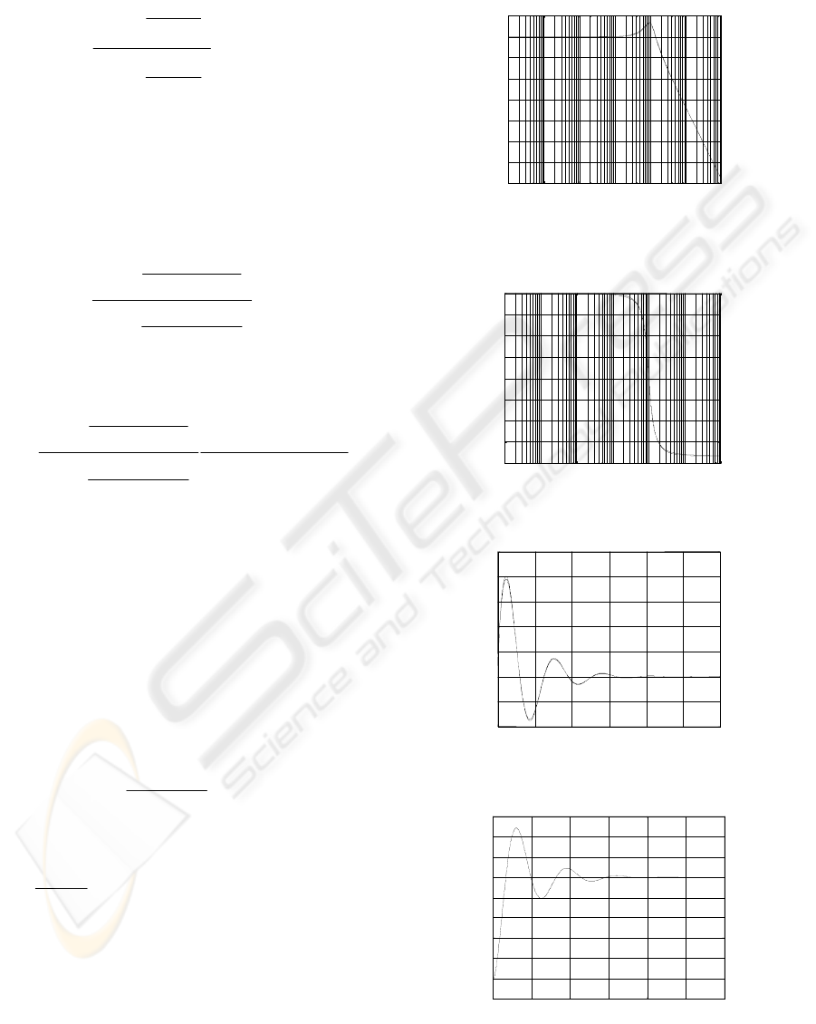
Figures (5) and (6) show the Bode plots of the
system transfer function and its proposed rational
function approximation. Figures (7) and (8) show
respectively the impulse and the step responses of
the system obtained from its proposed rational
function approximation.
4 CONCLUSION
In this paper I have presented some effective
methods for approximating the irrational function
given by
])s(1[
1
)s(G
m
0
τ+
=
, for 0 < m < 2,
representing the transfer function of the fundamental
linear fractional order differential equation
)t(e)t(x
dt
)t(xd
)(
m
m
m
0
=+τ
by a rational function, in
a given frequency band. The impulse and step
responses of this type of systems are derived.
Illustrative examples have been treated to
demonstrate the usefulness of the approximation
methods.
Theses approximations can very suitable for
analysis, realization and implementation of
fractional order systems. The expressions for
characteristics and usual time and frequency
specifications can also be derived.
Figure 5: Magnitude Bode plot.
Figure 6: Phase of the Bode plot.
Figure 7: Impulse response.
Figure 8: Step response.
10
-3
10
-2
10
-1
10
0
10
1
10
2
10
3
-70
-60
-50
-40
-30
-20
-10
0
10
Frequency (Rad/s)
Magnitude (dB)
10
-3
10
-2
10
-1
10
0
10
1
10
2
10
3
-160
-140
-120
-100
-80
-60
-40
-20
0
Frequency (Rad/s)
Phase (deg)
0
0.5
1
1.5
2
2.5
3
-4
-2
0
2
4
6
8
10
Time (sec)
Amplitude
0
0.5
1
1.5
2
2.5
3
-0.2
0.0
0.2
0.4
0.6
0.8
1.0
1.2
1.4
1.6
Amplitude
Time (sec)
ICINCO 2007 - International Conference on Informatics in Control, Automation and Robotics
412

REFERENCES
Torvik, P.J. and Bagley, R. L.,1984, ‘On the Appearance
of the Fractional Derivative in the Behavior of Real
Materials,’ Transactions of the ASME, vol. 51.
Ichise, M., Nagayanagi, and Y., Kojima, T., 1971 “An
Analog Simulation of Non-Integer Order Transfer
Functions for Analysis of Electrode Processes,” J. of
Electro-analytical Chemistry, vol. 33.
Sun, H.H. and Onaral, B., 1983, ‘A Unified Approach to
Represent Metal Electrode Polarization,’ IEEE
Transactions on Biomedical Engineering, vol. 30.
Cole, K.S. and Cole, R.H., 1941, ‘Dispersion and
absorption in dielectrics, alternation current
characterization,’ Journal of Chem. Physics vol. 9.
Davidson, D. and Cole, R., 1950, ‘Dielectric relaxation in
glycerine,’ J. Chem. Phys., vol.18.
Manabe, S., 1961, ‘The Non-Integer Integral and its
Application to Control Systems,’ ETJ of Japan, vol. 6,
N° 3-4.
Oustaloup, A., 1983, Systèmes Asservis Linéaires d’Ordre
Fractionnaire : Théorie et Pratique-, Editions Masson,
Paris.
Charef, A., Sun, H. H., Tsao, Y.Y., and Onaral, B., 1992,
‘Fractal system as represented by singularity function,’
IEEE Transactions on Automatic Control, Vol. 37,
N°9.
Podlubny, I., 1994, ‘Fractional-order Systems and
fractional-Order Controllers,’ UEF-03-94 Slovak
Academy of Science, Kosice.
Miller, K.S. and Ross, B., 1993, An Introduction to the
Fractional Calculus and Fractional Differential
Equations, John Wiley & Sons Inc., New-York.
Hartley, T.T. and Lorenzo C. F., 1998, ‘A solution of the
fundamental linear fractional order differential
equation,’ NASA TP-1998-208693, December 1998
Petras, I., Podlubny, I., O’Leary, P., Dorcak, L., and
Vinagre, B. M., 2002, ‘Analogue Realization of
Fractional Order Controllers,’ Fakulta Berg , TU
Kosice.
MacDonald, J.R., 1987, Impedance spectroscopy, John
Wiley, New York.
Sun, H. H., Charef, A., Tsao, Y.Y., and Onaral, B., 1992,
‘Analysis of Polarization Dynamics by Singularity
Decomposition Method,’ Annals of Biomedical
Engineering, Vol. 20.
Kuo, Benjamin C., 1987, Automatic control systems,
Englewood Cliffs, Prentice-Hall, Englewood Cliffs,
New Jersey.
SOLUTION OF THE FUNDAMENTAL LINEAR FRACTIONAL ORDER DIFFERENTIAL EQUATION
413