COLLABORATIVE CONTROL IN A HUMANOID DYNAMIC TASK

Diego Pardo and Cecilio Angulo

GREC - Knowledge Engineering Research Group

UPC - Technical University of Catalonia

Avda. Victor Balaguer s/n. Vilanova i la Geltr

u, Spain

Keywords:

Robot control architecture, Sensorimotor learning, Coordination policy, Reinforcement learning.

Abstract:

This paper describes a collaborative control scheme that governs the dynamic behavior of an articulated mobile

robot with several degrees of freedom (DOF) and redundancies. These types of robots need a high level of co-

ordination between the motors performance to complete their motions. In the employed scheme, the actuators

involved in a speciﬁc task share information, computing integrated control actions. The control functions are

found using a stochastic reinforcement learning technique allowing the robot to automatically generate them

based on experiences. This type of control is based on a modularization principle: complex overall behavior

is the result of the interaction of individual simple components. Unlike the standard procedures, this approach

is not meant to follow a trajectory generated by a planner, instead, the trajectory emerges as a consequence

of the collaboration between joints movements while seeking the achievement of a goal. The learning of the

sensorimotor coordination in a simulated humanoid is presented as a demonstration.

1 INTRODUCTION

Robots with several Degrees of Freedom (DOF) and

redundant conﬁgurations are more frequently con-

structed; humanoids like Qrio (Kuroki et al., 2003),

Asimo (Hirai et al., 1998) or HRP-2 (Kaneko et al.,

2004), and entertainment robots like Aibo (Fujita and

Kitano, 1998) are examples of it. Complex move-

ments in complex robots are not easy to calculate, the

participation of multiple joints and its synchroniza-

tion requirements demands novel approaches that en-

dow the robot with the ability of coordination. An

attempt to drive the dynamics of its body optimally,

measuring its performance in every possible conﬁg-

uration, would bring to a combinational explosion of

its solution space.

The habitual use of simpliﬁed mathematical mod-

els to represent complex robotic systems, i.e., approx-

imating non-linearities and uncertainties, would result

in policies that execute approximately optimal con-

trol, thus, two major assumptions command the devel-

oped work. First, there is no pre-established mathe-

matical model of the physics of the robot’s body from

which a control law could be computed; and second,

the control design philosophy is focused on the ac-

tion performance of the robot and not on the trajectory

achievement by its joints; as an alternative, stochastic

reinforcement learning techniques applied to numeri-

cal simulation models are studied. An optimal control

problem, where a cost function is minimized to com-

pute the policies, is stated.

The goal of this work is to solve a multi-joint robot

motion problem where coordination is need. Plan-

ners and trajectory generators are usually in charge of

complex motions where many joints are involved and

the mechanical stabilization of the robot is in risk; the

relationship between sensory signals and motor com-

mands at the level of dynamics is viewed as a low

level brick in the building of control hierarchy. Here

we use a dynamic control scheme that also solves the

trajectory problem.

It is important to mention that a previous work

uses coordination at the level of dynamics to extend

a manipulator robot capacity (Rosenstein and Barto,

2001), their objective was to use a biologically in-

spired approach to proﬁt synergical movements be-

tween joints, like human muscles relationship. They

use a hand-made pre-established PID controllers in

174

Pardo D. and Angulo C. (2007).

COLLABORATIVE CONTROL IN A HUMANOID DYNAMIC TASK.

In Proceedings of the Fourth International Conference on Informatics in Control, Automation and Robotics, pages 174-180

DOI: 10.5220/0001629001740180

 SciTePress

every joint of the robot and the ﬁnal applied torque

in each motor is the linear combination of the PID’s

output, then collaboration is shown. The combina-

tion parameters are obtained by direct search meth-

ods (Rosenstein, 2003). By using linear controllers

to solve a nonlinear problem, they implement a hi-

erarchical motor program that runs various feedback

controllers, i.e, they switch between PID’s (parame-

ters and goal) in the middle of the motion.

Here we extend that result by proposing a more

general scheme, where sensor information is pro-

cessed in independent and speciﬁc layers to produce

coordinate control actions. Furthermore, at the ar-

chitecture deﬁnition, the control functions are no re-

stricted to PID’s and its linear combination. Addition-

ally, we use reinforcement learning to compute all the

architecture controllers.

This paper is organized as follows Section 2 is de-

voted to the presentation of the architecture and a lin-

ear implementation of practical use is outlined in 3;

while section 4 validates it through a simulation ex-

periment of a robot equilibrium dynamical task. Sec-

tion 6 gathers the conclusions and points to the future

work.

2 LAYERED COOPERATIVE

CONTROL

The Layered Cooperative Control (LCC) scheme is

meant to generate motions while solving a Dynamical

Task (DT). It is assumed that the ﬁnal conﬁguration of

the DT is known, i.e. the set point of the joints angles

is preestablished; but how to coordinate motions to

reach this conﬁguration, restricted to its body dynam-

ics, is unknown. It is also assumed that the states of

the system are observable and that each joint position

is commanded by independent servos.

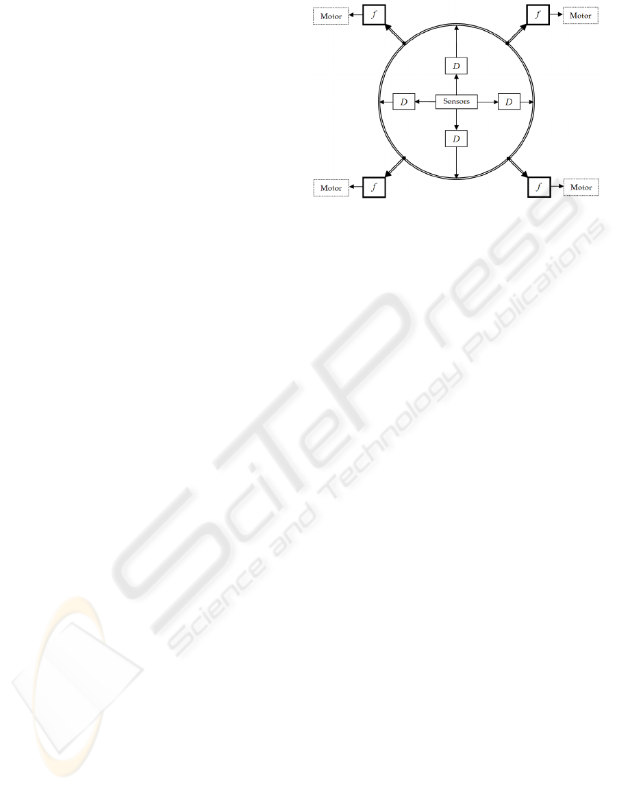
Figure 1 represents schematically the main idea

of the LCC. The control actions that drive the motors

are processed by two layers of controller functions.

Each component of the ﬁrst layer (D) manipulates the

dynamics of a singular joint; the output of this layer

intends to position its corresponding joint in a pre-

viously speciﬁed angle, but it is ﬁltered by the sec-

ond layer of controllers ( f ). Each motor is driven by

a different function, which calculates the control ac-

tion based on all the signals originated in the previous

layer.

The controllers of the ﬁrst layer are related with

the dynamics of the link, they must be established

once. The second layer of functions ( f ) must be de-

signed facing the DT intended to be completed. Func-

tionally and computationally speaking the architec-

Figure 1: LCC Basic Idea : Two layers of control.

ture is layered; every time step two mappings take

place, one for error position reasons and the other

seeking coordination between joints.

Every controller of the second layer ( f ) uses the

information originated in all the ﬁrst layer’s con-

trollers. This collaboration allows joint controllers to

know the dynamical state of the others, and then to

act according to it in order to complete the DT.

2.1 Architecture Formulation

Let the articulated mobile robot have n joints. Each

joint has an error based controller D

with (i = 1, ..., n)

in the ﬁrst layer. This is a SISO function, whose input

is the error of the position of its respective joint (e

)

and whose output is a control action (u

). The error is

calculated using the sensor information providing the

actual position of the joint (θ

) and the already known

set point or goal conﬁguration (θ

∗

= θ

− θ

∗

= D

) i = 1, ..., n

Let the dynamical task have associated n controllers f

in the second layer with (i = 1, ..., n), these are MISO

functions whose inputs are the n outputs u

of the ﬁrst

layer described above. The output of the second layer

functions v

is the velocity applied on the correspond-

ing motor (M

= f

, ..., u

) i = 1, ..., n

The robot state is represented by a continuous time

dynamical system controlled by a parameterized pol-

icy,

˙x = g(x, v) + h(x) · v (1)

v = π

(x, v) (2)

where vector x represents the states of the robot, g and

h its dynamics, v the control action and π the control

policy parameterized by the vector w.

COLLABORATIVE CONTROL IN A HUMANOID DYNAMIC TASK

175

2.2 LCC Synthesis

Once the control scheme has been stated, the next

step is the deﬁnition of a methodology to compute the

functions ( f

, D

). Here a policy gradient reinforce-

ment learning (PGRL) algorithm is employed. PGRL

methods (see (Williams, 1992),(Sutton et al., 2000))

are based on the measurement of the performance of

a parameterized policy π

applied as control function

during a delimited amount of time. In order to mea-

sure the performance of the controller, the following

function is deﬁned,

V (w) := J(x, π

(x)) (3)

where the measurement of the performance V of the

parameters w is done by deﬁning the cost function J.

By restricting the scope of the policy to certain

class of parameterized functions u = π

(x), the per-

formance measure (3) is a surface where the maxi-

mum value corresponds to the optimal set of param-

eters w ∈ R

. The search for the maximum can be

performed by standard gradient ascent techniques,

k+1

= w

+ η∇

V (w) (4)

where η is the step size and ∇

V (w) is the gradient

of V (w) with respect to w. The analytical formulation

of this gradient is not possible without the acquisition

of a mathematical model of the robot. The numeri-

cal computation is also not evident, then, a stochastic

approximation algorithm is employed : the ‘weight

perturbation’ (Jabri and Flower, 1992), which esti-

mates the unknown gradient using a Gaussian random

vector to orientate the change in the vector parame-

ters. This algorithm is selected due to its good per-

formance, easy derivation and fast implementation;

note that the focus of this research is not the choice

of a speciﬁc algorithm, nor the development of one,

but rather the cognitive architecture to provide robots

with the coordination learning ability.

This algorithm uses the fact that, by adding to w

a small Gaussian random term z with E{z

} = 0 and

E{z

} = σ

i j

, the following expression is a sample

of the desired gradient

α(w) = [J(w + z) − J(w)]· z (5)

Then, both layers’ controllers can be found using this

PGRL algorithm.

= D

) (6)

= f

, ..., u

)

In order to be consequent with the proposed deﬁnition

of each layer, the training of the vector parameters

must be processed independently; ﬁrst the dynami-

cal layer and then the coordination one. It is assumed

that the movement has to take place between a limited

amount of time T , where signals are collected to com-

pute the cost function (3), then, the gradient is esti-

mated using (5) and a new set of parameters obtained

applying the update strategy of (4). Notice that in the

case of the ﬁrst layer, each function D

is trained and

updated separately from the others of the same layer,

but when learning the coordinate layer, all the func-

tions f

must be updated at the same time, because

in this case the performance being measured is that of

the whole layer.

3 LINEAR IMPLEMENTATION

The previous description of the LCC is too general

to be of practical use. Then, it is necessary to make

some assumptions about the type of functions to be

used as controllers. A well known structure to control

the dynamic position of one link is the Proportional

Integral Derivative (PID) error compensator. It has

the following form,

= K

· e

+ K

· e

dt (7)

The functionality of its three terms (K

, K

) of-

fers management for both transient and steady-state

responses, therefore, it is a generic and efﬁcient so-

lution to real world control problems. By the use

of this structure, a link between optimal control and

PID compensation is revealed to robotic applications.

Other examples of optimization based techniques for

tuning a PID are (Daley and Liu, 1999; Koszalka

et al., 2006).

The purpose of the second layer is to compute the

actual velocity to be applied on each motor by gath-

ering information about the state of the robot while

processing a DT. The PID output signals are collected

and ﬁltered by this function to coordinate them. Per-

haps the simplest structure to manage this coordina-

tion is a gain row vector W

, letting the functions in

the second layer be the following,

(u) = W

· u

Then, a linear combination of u commands the coor-

dination. The matrix W

encapsules all the infor-

mation about this layer for the mth DT.







. . . w







(8)

Where the term w

i j

is the speciﬁc weight of the jth

PID in the velocity computation of the joint i.

ICINCO 2007 - International Conference on Informatics in Control, Automation and Robotics

176

4 HUMANOID COORDINATION

Classical humanoid robot motions are typically very

slow in order to maintain stability; e.g., the biped

walking based on Zero Moment Point (ZMP) (Vuko-

bratovic and Stepanenko, 1972) condition avoids

those states far from the pre-determined trajectory in

which the momentum is guaranteed. By doing this,

thousands of trajectories and capabilities of the robot

could be restricted. Highly dynamic capabilities need

those avoided states to perform quick and realistic

motions.

4.1 The Simulation Robot Environment

A simulated humanoid is employed as a test-bed to

evolve the controllers. It was modeled using Webots

(Michel, 2004), a 3D robot simulation platform . De-

tails can be obtained in (Webots, ).

This particular model of the full body humanoid

robot has a total of 25 DOF, each link torque is limited

to [−10, 10] Nm, additionally it has a camera, a dis-

tance sensor, a gps, 2 touch sensors in the feet, and a

led in the forehead. The model includes physical char-

acteristics; the software processes kinematic and dy-

namic simulation of the interaction between the robot

and its environment.

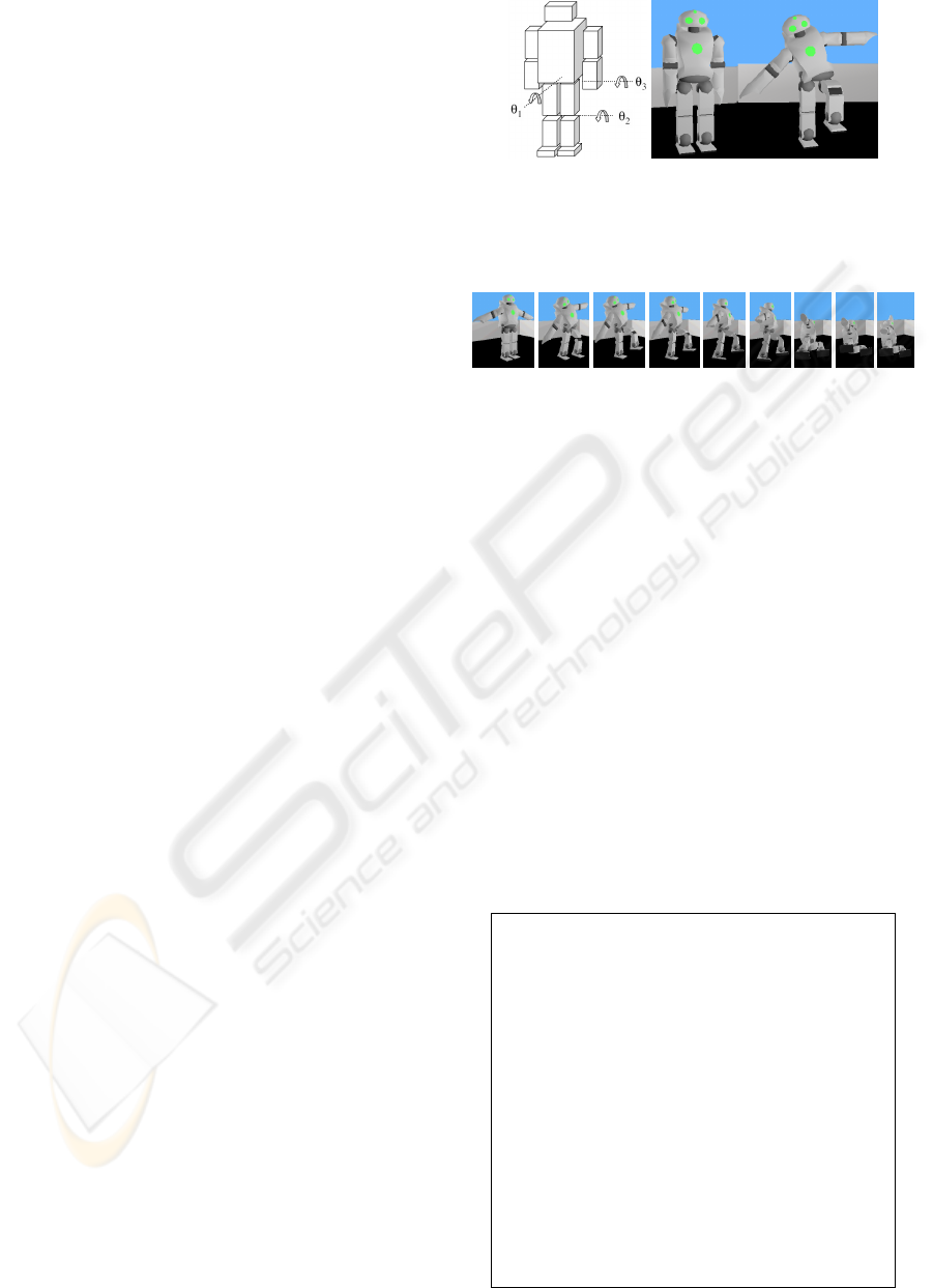
4.2 The One-Leg Equilibrium Task

The goal of the simulation experiment is to reach a

ﬁnal conﬁguration called ’one-leg equilibrium point’

starting from the passive stand up position. Three

joints are involved in this motion (see Figure 2(a).):

The longitudinal axis of the Back, the transversal axis

of the left hip and the left knee; their goal states,

i.e. angles in radians, are θ

∗

= 0.4, θ

∗

= 1.5 and

∗

= 1.5 respectively, with ﬁnal velocity

∗

= 0 for

all the joints. Both conﬁgurations, initial and ﬁnal,

are shown in Figure 2(b). The goal conﬁguration has

been designed to generate a slight inclination of the

back to the right side, changing the center of mass of

the body of the robot, thus, letting more weight sup-

ported on the right leg, and then allowing the left leg

to lift, by means of the blending of the hip and knee

articulations.

Figure 3 shows the simulation sequence of the mo-

tion of the robot using standard low level controllers.

The robot falls down when attempts to reach the goal

conﬁguration due to the forces generated by the fric-

tion between the ﬂoor and its foot soles. The whole

body of the robot suffers a destabilization at the start

of the movement.

(a) (b)

Figure 2: Simulated Humanoid (a). Joints involved in the

motion. (b) Initial and goal conﬁguration.

Figure 3: Direct Solution: Failure Demonstration.

4.3 The Learning Procedure

Table 1 shows the PGRL algorithm. A supervisor pro-

gram is in charge of the training; its EVALUATE sub-

routine delivers the set of values to be evaluated in

the robot controllers. It starts a controlled episode

from the initial conﬁguration and intends to achieve

the goal states; every evaluation takes T = 12s, within

this time the cost function is measured and returned.

The supervisor repeats this operation until a conver-

gence criterium is matched or the number of iterations

is too large.

In this experiment the PID values are learned but not

calculated. The following is the discrete implementa-

Table 1: Weight perturbation PGRL Algorithm.

input

step size η ∈ [0, 1]

search size σ ≥ 0

max step ∆

max

∈ [0, 1]

initialize

← I ∈ R

3×3

(Identity Matrix)

α ← 0

J ← EVALUATE(W)

repeat

1. z ← N(0, σ)

3. J

← EVALUATE(W+z)

4. α ← [J

− J] · z

5. ∆W ← −ηα

6. ∆W ← min(∆W, ∆

max

)

7. W ← W + ∆W

8. J ←EVALUATE(W)

until convergence or number of iterations too large

return W, J

COLLABORATIVE CONTROL IN A HUMANOID DYNAMIC TASK

177

tion of the PID employed,

= K

· e

+ K

· (e

− e

t−1

) + K

∑

j=0

(9)

Where u

represents the control signal associated with

joint i at step time t, it depends on its corresponding

position error e

= θ

∗

− θ

. This controller must pro-

vide zero position error in a single joint motion, there-

fore its parameters are learned using as performance

criteria the following expression,

(V ) = −

∑

t=0

(θ

∗

− θ

)

∑

t=0

(

)

(10)

The PID is tested using a time step of ∆T = 32ms

during T = 12s. The algorithms constants used are

σ = 0.032 and η = 0.05. For the learning of the par-

ticular PID in charge of controlling the back, special

restrictions are implemented to the reward function,

penalizing those episodes where the robot falls down.

The penalization is proportional to the time the robot

stays on the ground.

The linear parameterized function selected for the

coordination layer is:

= W · u

(11)

where v

∈ ℜ

are the actual ﬁnal velocities; u

∈ ℜ

the outputs of the PIDs; and W ∈ ℜ

3×3

is the transfor-

mation that contains the parameters to be found (W

i j

The algorithm starts with a diagonal matrix as co-

ordination controller, i.e. W

= I, meaning that the

ﬁrst collaborative control function attempted is that in

which just the original PID controllers act. The non-

diagonal values of K deliver coordination. Same algo-

rithms constants and time step are used in this stage

of the LCC implementation.

5 RESULTS

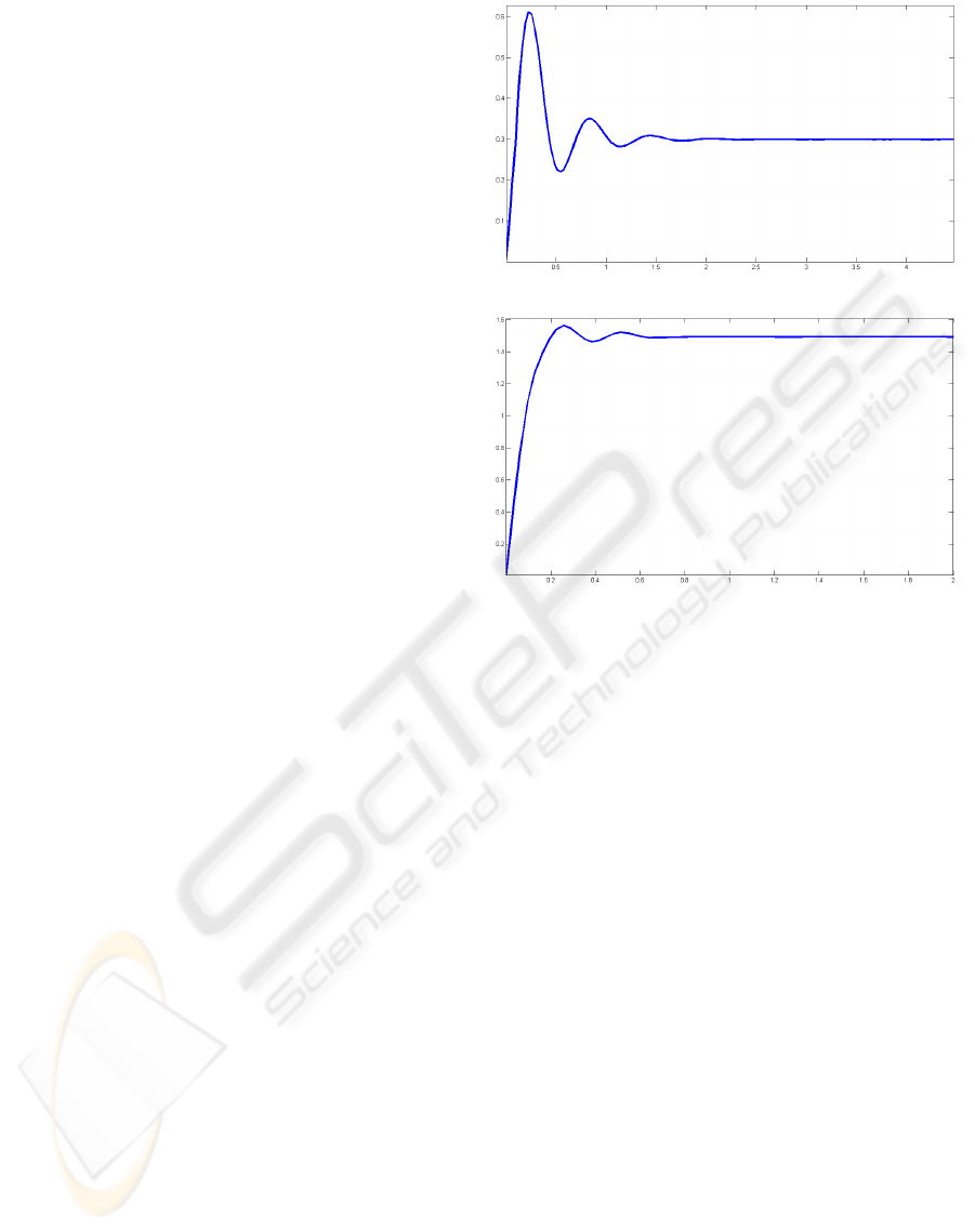
5.1 PID Controller

Several local minima are found. Figure 4(a) shows the

output of the back joint using one of the PID solutions

found. It presents big overshoot, but no stationary er-

ror to a set point of θ

∗

= 0.3, and mainly: The robot

learns how ’not to fall’.

The behavior of the Back joint is equivalent with an

inverted pendulum system with a big mass being ma-

nipulated (robot torso). For this joint, and for a better

controlled output, a more complex parameterized pol-

icy would be needed. On the other hand, Figure 4(b)

presents the output of the hip joint. It is evident that

(a)

(b)

Figure 4: (a) Back-Joint position output (radians), using a

learned PID (set point=0.3rad), (b) Hip-Joint position out-

put (radians) using a learned PID (set point=1.5rad).

a better solution is achieved, this is because the train-

ing of this PID is done in a lay down position, with

no risk of falling, and the mass of the link being con-

trolled is widely insigniﬁcant compared with that in

the back-joint case.

Final values for the independent joints controllers

(Back, Hip and Knee) are :

PID

= [0.746946 0.109505 0.0761541]

PID

= [0.76541 0.0300045 0]

PID

= [0.182792 0.0114312 0.00324704]

5.2 Coordination Layer

After several iterations, the best solution is found; a

sequence of the humanoid learned motion is depicted

in Figure 5. The associate coordination controller is

the following:

W =





0.6612900 −0.3643360 −0.1936260

−0.0497653 1.0266600 −0.0684569

0.0285586 0.1469820 0.9642390





Note how the non-diagonal parameters have grown,

allowing the coordination. This characteristic has

ICINCO 2007 - International Conference on Informatics in Control, Automation and Robotics

178

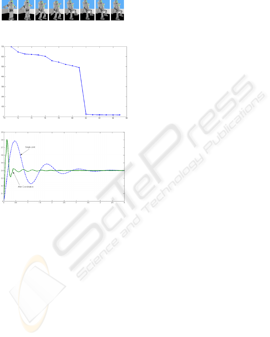
Figure 5: Simulated Humanoid One-Leg Equilibrium task.

(a)

(b)

Figure 6: (a) Reward Evolution J(W ) of the best learned so-

lution (last 20 tirals); (b) Back-joint position, before (dotted

line) and after the coordination learning.

been previously pointed out in (Rosenstein and Barto,

2001), but here in an unstable 3D system task.

For this particular solution, the evolution of the

reward is presented in Figure 6(a). Once the robot

learns how ‘not to fall’ the convergence rate increases

and the ﬁnal results get to lower values.

It is important to mention that the robot presents

some absolute displacement, tending to go back-

wards. A better designed reward function is needed

to avoid absolute displacements, but a good solution

is harder to ﬁnd in this scenario. Finally, it is impor-

tant to emphasize the change in the behavior of the

back joint after the second layer phase. It seems like

the system learns that the overshoot must be shorter in

time in order to be able to lift the leg with out falling

down. Figure 6(b). shows the output of the back joint

before and after the second layer of learning.

6 CONCLUSIONS

The LLC scheme proposes to use the dynamic inter-

action of the robots articulations as a trajectory gen-

erator, without the use of a trajectory planner. Ex-

ploiting dynamics gives the robot the ability to ex-

plore motion interactions that result in optimized be-

haviors: Learning at the level of dynamics to succeed

in coordination.

The presented solution overcomes the model de-

pendency pointed above; by the presentation of a sys-

tematic control scheme the ideas of (Rosenstein and

Barto, 2001) are extended. Here, the low level con-

trollers are found using learning techniques and the

formulation of a control architecture allows the im-

plementation of different parameterized policies.

The interaction between Machine Learning, Con-

trol Systems and Robotics creates an alternative for

the generation of artiﬁcial systems that consistently

demonstrate some level of cognitive performance.

Currently, highly dynamic motions in humanoids

are widely unexplored. The capability of this robots

will be extended if motions that compromise the

whole-body dynamic are explored. The LCC is tested

within a simulated humanoid and succeed in the per-

formance of a very fast motion, one in which the

whole-body equilibrium is at risk.

Coordination is possible thanks to the sharing of

information.

ACKNOWLEDGEMENTS

This work has been partly supported by the Spanish

MEC project ADA (DPI2006-15630-C02-01). Au-

thors would like to thank Olivier Michel and Ricardo

Tellez for their support and big help.

REFERENCES

Daley, S. and Liu, G. (1999). Optimal pid tuning using

direct search algorithms. Computing and Control En-

gineering Journal, 10(2):251–56.

Fujita, M. and Kitano, H. (1998). Development of an au-

tonomous quadruped robot for robot entertainment.

Autonomous Robots, 5(1):7–18.

Hirai, K., Hirose, M., Haikawa, Y., and Takenaka, T. (1998).

The development of honda humanoid robot. In Pro-

ceedings of the IEEE International Conference on

Robotics and Automation, ICRA.

Jabri, M. and Flower, B. (1992). Weight perturbation: An

optimal architecture and learning technique for analog

VLSI feedforward and recurrent multilayer networks.

COLLABORATIVE CONTROL IN A HUMANOID DYNAMIC TASK

179

IEEE Transactions on Neural Networks, 3(1):154–

157.

Kaneko, K., Kanehiro, F., Kajita, S., Hirukawa, H.,

Kawasaki, T., Hirata, M., Akachi, K., and Isozumi,

T. (2004). Humanoid robot hrp-2. In Proceedings of

the IEEE International Conference on Robotics and

Automation, ICRA.

Koszalka, L., Rudek, R., and Pozniak-Koszalka, I. (2006).

An idea for using reinforcement learning in adaptive

control systems. In Proceedings of the IEEE Int Con-

ference on Networking, Systems and Mobile Com-

munications and Learning Technologies, Kerkrade,

Netherlands.

Kuroki, Y., Blank, B., Mikami, T., Mayeux, P., Miyamoto,

A., Playter, R., Nagasaya, K., Raibert, M., Nagano,

M., and Yamaguchi, J. (2003). A motion creating sys-

tem for a small biped entretainment robot. In Proceed-

ings of the IEEE International Conference on Intelli-

gent Robots and Systems, IROS.

Michel, O. (2004). Webots: Professional mobile robot

simulation. Journal of Advanced Robotics Systems,

1(1):39–42.

Rosenstein, M. T. (2003). Learning to exploit dynamics for

robot motor coordination. PhD thesis, University of

Massachusetts, Amherst.

Rosenstein, M. T. and Barto, A. G. (2001). Robot

weightlifting by direct policy search. In Proceedings

of the IEEE International Conference on Artiﬁcial In-

telligence, IJCAI, pages 839–846.

Sutton, R., McAllester, D., Singh, S., and Mansour, Y.

(2000). Policy gradient methods for reinforcement

learning with function approximation. Advances in

Neural Information Processing Systems, 12:1057–

1063.

Vukobratovic, M. and Stepanenko, J. (1972). On the stabil-

ity of anthropomorphic systems. Mathematical Bio-

sciences, 15:1–37.

Webots. http://www.cyberbotics.com. Commercial Mobile

Robot Simulation Software.

Williams, R. J. (1992). Simple statistical gradient-following

algorithms for connectionist reinforcement learning.

Machine Learning, 8:229–256.

ICINCO 2007 - International Conference on Informatics in Control, Automation and Robotics

180