METRICS FOR MEASURING DATA QUALITY

Foundations for an Economic Data Quality Management

Bernd Heinrich, Marcus Kaiser and Mathias Klier

Department of Information Systems & Financial Engineering, University of Augsburg

Universitätsstr. 16, Augsburg, Germany

Keywords: Data Quality, Data Quality Management, Data Quality Metrics.

Abstract: The article develops metrics for an economic oriented managemen

t of data quality. Two data quality dimen-

sions are focussed: consistency and timeliness. For deriving adequate metrics several requirements are

stated (e. g. normalisation, cardinality, adaptivity, interpretability). Then the authors discuss existing ap-

proaches for measuring data quality and illustrate their weaknesses. Based upon these considerations, new

metrics are developed for the data quality dimensions consistency and timeliness. These metrics are applied

in practice and the results are illustrated in the case of a major German mobile services provider.

1 INTRODUCTION

In recent years data quality (DQ) has – due to an

extended use of data warehouse systems, coopera-

tive information systems (Cappiello et al., 2003) and

a higher relevance of customer relationship man-

agement – gained more and more importance in sci-

ence and practice. This refers to the fact that – for

decision makers – the benefit of data depends heav-

ily on completeness, correctness, consistency and

timeliness. These properties are known as DQ di-

mensions (Wang et al., 1995). Many firms have

problems to ensure DQ (Strong et al., 1997) and

according to a study by Redman (Redman, 1998)

“the total cost of poor data quality” is between 8 and

12 percent of their revenues. Moreover, an often

cited survey by the DW Institute revealed poor DQ

damaging US economy for more than 600 billions

US-$ per year (The Data Warehousing Institute,

2002). Other statistics indicate that 41 percent of the

data warehouse projects fail, mainly due to insuffi-

cient DQ (Meta Group, 1999). 67 percent of market-

ing managers think that the satisfaction of their cus-

tomers suffers from poor DQ (SAS Institute, 2003).

These figures illustrate impressively the relevance of

DQ nowadays. The consequences of poor DQ are

manifold: They range from worsening customer re-

lationships and customer satisfaction by incorrect

addressing of customers to a bad decision support of

managers.

The growing relevance of DQ re

vealed the need

for adequate measurement. Quantifying the current

state of DQ (e. g. of a data base) is essential for

planning DQ measures in an economic manner.

In the following we discuss how metrics for se-

ected DQ dimensions can be developed with regard

to two objectives:

a) Ena

bling the measurement of DQ

b) Anal

ysing the consequences of DQ measures

(e. g. data cleansing of customer’s address data

improving the quantified correctness)

The developed metrics were applied in coopera-

tio

n with a major German mobile services provider.

The objective of the project was to analyse the eco-

nomic consequences of DQ measures in the case of

campaign management. The following questions

were relevant within the project:

• Ho

w can DQ be quantified and measured by

means of metrics?

• How ca

n DQ measures improve these metrics

and what are the economic consequences?

The paper is organised as follows: The next sec-

ion defines requirements on DQ metrics. In sec-

tion 3 selected approaches are discussed. Section 4

develops new metrics for the DQ dimensions consis-

tency and timeliness, and examines their advantages.

A discussion of how the metric for timeliness was

applied within the campaign management of a mo-

bile services provider can be found in section 5. The

Heinrich B., Kaiser M. and Klier M. (2007).

METRICS FOR MEASURING DATA QUALITY - Foundations for an Economic Data Quality Management.

In Proceedings of the Second International Conference on Software and Data Technologies - Volume ISDM/WsEHST/DC, pages 87-94

DOI: 10.5220/0001325600870094

 SciTePress

last section sums up and reflects critically the re-

sults.

2 REQUIREMENTS ON DATA

QUALITY METRICS

Applying an economic DQ management in practice,

metrics are needed for quantifying DQ in order to

answer questions like the following: Which measure

improves DQ most and which one has the best bene-

fit/costs ratio?

Figure 1 illustrates the closed loop of an eco-

nomic oriented management of DQ. This loop can

be influenced via DQ measures. Taking measures

improves the current level of DQ (quantified by

means of metrics). This leads to a corresponding

economic benefit (e. g. enabling a more effective

customer contact). Moreover, based on the level of

DQ and taking into account benchmarks and thresh-

olds, firms can decide on taking (further) measures

or not. From an economic view, only those measures

must be taken that are efficient with regard to costs

and benefit (Campanella, 1999; Feigenbaum, 1991;

Machowski & Dale, 1998; Shank & Govindarajan,

1994). E. g. given two measures having equal eco-

nomic benefit, it is rational to choose the one with

lower costs.

dimensions

measure

costs

benefit

Kennzahl

metrics

dimensions

measure

costs

benefit

Kennzahl

metrics

measure

costs

benefitbenefit

Kennzahl

metrics

Kennzahl

metrics

Figure 1: Data quality loop.

Therefore, this paper aims at quantifying the

quality of a dataset by means of metrics for particu-

lar dimensions. The identification and classification

of DQ dimensions is treated by many publications

from both, a scientific and a practical point of view

(English, 1999; Eppler, 2003; Helfert, 2002; Lee et

al., 2002; Jarke & Vassiliou, 1997; Redman, 1996).

In the following, we focus on two dimensions for

illustrational purposes: consistency and timeliness.

Within an economic oriented DQ management sev-

eral requirements on DQ metrics can be stated for

enabling a practical application (cp. Even &

Shankaranarayanan, 2005; Hinrichs, 2002):

R1: [Normalisation] An adequate normalisation is

necessary for assuring the results being inter-

pretable and comparable.

R2: [Cardinality] For supporting economic evalua-

tion of measures, we require cardinality (cp.

White, 2006) of the metrics.

R3: [Adaptivity] For measuring DQ in a goal-

oriented way, it is necessary, that the metrics

can be adapted to a particular application.

R4: [Ability of being aggregated] In case of a rela-

tional database system, the metrics shall allow a

flexible application. Therefore, it must be possi-

ble to measure DQ at the layer of attribute val-

ues, tupels, relations and the whole database. In

addition, it must be possible to aggregate the

quantified results on a given layer to the next

higher layer.

R5: [Interpretability] Normalisation and cardinality

are normally not sufficient in practical applica-

tions. In fact, the DQ metrics have to be inter-

pretable, comprehensible and meaningful.

The next section reviews the literature consider-

ing the requirements listed above. Moreover it pro-

vides an overview over selected metrics.

3 LITERATURE ON MEASURING

DATA QUALITY

The literature already provides several approaches

for measuring DQ. They differ in the DQ dimen-

sions taken into account and in the underlying meas-

urement procedures (Wang et al., 1995). In the fol-

lowing, we briefly describe some selected ap-

proaches.

The AIM Quality (AIMQ) method for measuring

DQ was developed at the Massachusetts Institute of

Technology and consists of three elements (Lee et

al., 2002): The first element is the product service

performance model which arranges a given set of

DQ dimensions in four quadrants. The DQ dimen-

sions are distinguished by their measurability de-

pending on whether the improvements can be as-

sessed against a formal specification (e. g. com-

pleteness with regard to a database schema) or a

subjective user’s requirement (e. g. interpretability).

On the other hand, a distinction is made between

product quality (e. g. correctness) and service quality

(e. g. timeliness). Based on this model, DQ is meas-

ured via the second element: A questionnaire for

asking users about their estimation of DQ. The third

element of the AIMQ method consists of two analy-

ICSOFT 2007 - International Conference on Software and Data Technologies

sis techniques for interpreting the assessments. The

first technique compares an organisation’s DQ to a

benchmark from a best-practices organisation. The

second technique measures the distances between

the assessments of different stakeholders.

Beyond novel contributions the AIMQ method

can be criticised for measuring DQ based on the

subjective estimation of DQ via a questionnaire.

This approach prohibits an automated, objective and

repeatable DQ measurement. Moreover, it provides

no possibility to adapt this measurement to a particu-

lar scope (R3). But instead it combines subjective

DQ estimations of several users who normally use

data for different purposes.

The approach by (Helfert, 2002) distinguishes -

based upon (Juran, 1999) - two quality factors: qual-

ity of design and quality of conformance (see also

Heinrich & Helfert, 2003). Quality of design denotes

the degree of correspondence between the users’

requirements and the information system’s specifica-

tion (e. g. specified by means of data schemata).

Helfert focuses on quality of conformance that

represents the degree of correspondence between the

specification and the information system. This de-

termination is important within the context of meas-

uring DQ: It separates the subjective estimation of

the correspondence between the users’ requirements

and the specified data schemata from the measure-

ment - which can be objectivised - of the correspon-

dence between the specified data schemata and the

existing data values. Helfert’s main issue is the inte-

gration of DQ management into the meta data ad-

ministration which shall enable an automated and

tool-based DQ management. Thereby the DQ re-

quirements have to be represented by means of a set

of rules that is verified automatically for measuring

DQ. However, Helfert does not propose any metrics.

This is due to his goal of describing DQ manage-

ment on a conceptual level.

Besides these scientific approaches two practical

concepts by English and Redman shall be presented

in the following. English describes the total quality

data management method (English, 1999) that fol-

lows the concepts of total quality management. He

introduces techniques for measuring quality of data

schemata and architectures (of an information sys-

tem), and quality of attribute values. Despite the fact

that these techniques have been applied within sev-

eral projects, a general, well-founded procedure for

measuring DQ is missing. In contrast, Redman

chooses a process oriented approach and combines

measurement procedures for selected parts in an

information flow with the concept of statistical qual-

ity control (Redman, 1996). He also does not present

any particular metrics.

From a conceptual view, the approach by

(Hinrichs, 2002) is very interesting, since he devel-

ops metrics for selected DQ dimensions in detail.

His technique is promising, because it aims at an

objective, goal-oriented measurement. Moreover this

measurement is supposed to be automated. A closer

look reveals that major problems come along when

applying Hinrichs’ metrics in practice, since they are

hardly interpretable. This fact makes a justification

of the metrics’ results difficult (cp. requirement R5).

E. g., some of the metrics proposed by Hinrichs - as

the one for consistency - base on a quotient of the

following form:

()

+function distance the of result

An example for such a distance function is

()

∑

ℜ

=1s

, where w denotes an attribute value within

the information system.

ℜ

is a set of consistency

rules (with |

ℜ

| as the number of set elements) that

shall be applied to w. Each consistency rule r

∈

ℜ

(s = 1, 2, …, |

ℜ

|) returns the value 0, if w fulfils the

consistency rule, otherwise the rule returns the value

Thereby the distance function indicates how many

consistency rules are violated by the attribute

value w. In general, the distance function’s value

range is [0; ∞]. Thereby the value range of the met-

ric (quotient) is limited to the interval [0; 1]. How-

ever, by building this quotient the values become

hardly interpretable relating to (R1). Secondly, the

value range [0; 1] is normally not covered, because a

value of 0 is resulting only if the value of the dis-

tance function is ∞ (e. g. the number of consistency

rules violated by an attribute value has to be infi-

nite). Moreover the metrics are hardly applicable

within an economic-oriented DQ management, since

both absolute and relative changes can not be inter-

preted. In addition, the required cardinality is not

given (R2), a fact hindering economic planning and

ex post evaluation of the efficiency of realised DQ

measures.

⎩

⎨

⎧

else1

ruley consistenc thefulfils if0

:)(

Table 1 demonstrates this weakness: For improving

the value of consistency from 0 to 0.5, the corre-

sponding distance function has to be decreased from

∞ to 1. In contrast, an improvement from 0.5 to 1

needs only a reduction from 1 to 0. Summing up, it

METRICS FOR MEASURING DATA QUALITY - Foundations for an Economic Data Quality Management

is not clear how an improvement of consistency (for

example by 0.5) has to be interpreted.

Table 1: Improvement of the metric and necessary change

of the distance function.

Improvement of

the metric

Necessary change of

the distance function

0.0 → 0.5 ∞ → 1.0

0.5 → 1.0 1.0 → 0.0

Besides, we have a closer look at the DQ dimen-

sion timeliness. Timeliness refers to whether the

values of attributes still correspond to the current

state of their real world counterparts and whether

they are out of date. Measuring timeliness does not

necessarily require any real world test. For example,

(Hinrichs, 2002) proposed the following quotient:

()()

1 valueattribute of age timeupdate attributemean

+⋅

This quotient bears similar problems like the pro-

posed metric for consistency. Indeed, the result tends

to be right (related to the input factors taken into

account). However, both interpretability (R5) – e. g.

the result could be interpreted as a probability that

the stored attribute value still corresponds to the

current state in the real world – and cardinality (R2)

are lacking.

In contrast, the metric defined for measuring

timeliness by (Ballou et al., 1998)

(

volatility

currency

]}0),1{max[(Timeliness −=

), can at

least – by choosing the parameter s = 1 – be inter-

preted as a probability (when assuming equal distri-

bution). But again, Ballou et al. focus on functional

relations – a (probabilistic) interpretation of the re-

sulting values is not provided.

Based on this literature reviews, we propose two

approaches for the dimensions consistency and time-

liness in the next section.

4 DEVELOPMENT OF DATA

QUALITY METRICS

According to the requirement R4 (ability of being

aggregated), the metrics presented in this section are

defined on the layers of attribute values, tupels, rela-

tions and database. The requirement is fulfilled by

constructing the metrics “bottom up”, i. e. the metric

on layer n+1 (e. g. timeliness on the layer of tupels)

is based on the corresponding metric on layer n (e. g.

timeliness on the layer of attribute values). Besides,

all other requirements on metrics for measuring DQ

defined above shall also be met.

First, we consider the dimension consistency:

Consistency requires that a given dataset is free of

internal contradictions. The validation bases on logi-

cal considerations, which are valid for the whole

data and are represented by a set of rules

ℜ

. That

means, a dataset is consistent if it corresponds to

ℜ

vice versa. Some rules base on statistical correla-

tions. In this case the validation bases on a certain

significance level, i. e. the statistical correlations are

not necessarily fulfilled completely for the whole

dataset. Such rules are disregarded in the following.

The metric presented here provides the advan-

tage of being interpretable. This is achieved by

avoiding a quotient of the form showed above and

ensuring cardinality. The results of the metrics (on

the layers of relation and data base) indicate the per-

centage share of the dataset considered which is

consistent with respect to the set of rules

ℜ

. In con-

trast to other approaches, we do not prioritise certain

rules or weight them on the layer of attribute values

or tupels. Our approach only differentiates between

either consistent or not consistent. This corresponds

to the definition of consistency (given above) basing

on logical considerations. Thereby the results are

easier to interpret.

Initially we consider the layer of attribute values:

Let w be an attribute value within the information

system and

ℜ

a set of consistency rules with |

ℜ

| as

the number of set elements that shall be applied to w.

Each consistency rule r

∈

ℜ

(s = 1, 2, …, |

ℜ

|) re-

turns the value 0, if w fulfils the consistency rule,

otherwise the rule returns the value 1:

Using r

⎩

⎨

⎧

else1

ruley consistenc thefulfils if0

:)(

(w), the metric for consistency is defined as

follows:

()()

∏

ℜ

−=ℜ

1:),(

sCons

wrwQ

(1)

The resulting value of the metric is 1, if the at-

tribute value fulfils all consistency rules defined in

ℜ

(i. e. r

(w) = 0 ∀ r

(w) ∈

ℜ

). Otherwise the result

is 0, if at least one of the rules specified in

ℜ

is vio-

lated. (i. e. ∃r

∈

ℜ

: r

(w) = 1). Such consistency

rules can be deducted from business rules or do-

main-specific functions, e. g. rules that check the

value range of an attribute (e. g.

00600 ≤ US zip code, US zip code ≤ 99950, US zip

ICSOFT 2007 - International Conference on Software and Data Technologies

code ∈ {0, 1, …, 9}

or marital status ∈ {“single”,

“married”, “divorced”, “widowed”}).

Now we consider the layer of tupels: Let T be a

tupel and

ℜ

the set of consistency rules r

(s = 1, 2, …, |

ℜ

|), that shall be applied to the tupel

and the related attribute values. Analogue to the

level of attribute values, the consistency of a tupel is

defined as:

()()

∏

ℜ

−=ℜ

1:),(

sCons

TrTQ

(2)

The results of formula (2) are influenced by rules

related to single attribute values and rules related to

several attribute values or the whole tupel. This en-

sures developing the metric “bottom-up“, since the

metric contains all rules related to attribute values.

I. e. if the attribute values of a particular tupel are

inconsistent with regard to the rules related to attrib-

ute values, this tupel can not be evaluated as consis-

tent on the layer of tupels. Moreover, if the attributes

of a particular tupel are consistent on the layer of

attribute values, this tupel may remain consistent or

become inconsistent on the layer of tupels. This de-

cision is made according to the rules related to tu-

pels.

In fact, a tupel is considered as consistent with

respect to the set of rules

ℜ

, if and only if all rules

are fulfilled (r

(T) = 0 ∀r

∈

ℜ

). Otherwise

Cons.

(T,

ℜ

) is 0, regardless whether one or several

rules are violated (∃r

∈

ℜ

: r

(T) = 1). Whereas

consistency rules on the layer of attribute values are

only related to a single attribute, consistency rules

on the layer of tupels can be related to different at-

tributes as e. g. (current date – date of birth < 14

years) ⇒ (marital status = “single”).

The next layer is the layer of relations: Let R be a

non-empty relation and

ℜ

a set of rules referring to

the attributes related. On the layer of relations the

consistency of a relation R can be defined via the

arithmetical mean of the consistency measurements

for the tupels T

∈ R (j = 1, 2, …, |T|) as follows:

),(

:),(

jCons

Cons

∑

ℜ

=ℜ

(3)

Finally, we consider the layer of data base: As-

sume D being a data base that can be represented as

a disjoint decomposition of the relations R

(k = 1, 2,

…, |R|). I. e., the whole database can be decomposed

into pair wise non-overlapping relations R

so that

each attribute of the database goes along with one of

the relations. Formally noted: D = R

∪ R

∪…

∪R

|R|

and R

∩ R

= ∅ ∀ i ≠ j. Moreover, let

ℜ

the set of rules for evaluating the consistency of the

data base. In addition,

ℜ

(k = 1, 2, …, |R|) is a dis-

joint decomposition of

ℜ

and all consistency rules

k,s

∈

ℜ

⊆

ℜ

concern only attributes of the relation

. Then the consistency of the data base D with

respect to the set of rules

ℜ

can be defined - based

on the consistency of the relations R

(k = 1, 2,

…, |R|) concerning the sets of rules

ℜ

- as follows:

()

∑

ℜ

=ℜ

),(

kkCons

Cons

gRQ

(4)

Whereas (Hinrichs, 2002) defines the consis-

tency of a data base by means of an unweighted ar-

ithmetical mean, the weights g

∈

[0; 1] allow to

incorporate the relative importance of each relation

depending on the given goal (R3). According to the

approach of Hinrichs, relations that are not that

much important for realising the goal are equally

weighted to relations of high importance. In addi-

tion, the metric’ results depends on the disjoint de-

composition of the database into relations. This

makes it difficult to evaluate objectively in the case

of using unweighted arithmetical mean. E. g., a rela-

tion R

with k ≠ 2 is weighted relatively with 1/n

when using the disjoint decomposition {R

, R

…, R

}, whereas the same relation is only weighted

with 1/(n+1) when using the disjoint decomposition

, R

', R

'', R

, …, R

} with R

∪

'' = R

and

∩

'' =

∅

Now, consistency can be measured by using the

metrics above in combination with corresponding

SQL queries for verifying the consistency rules. The

rules on the layers of attribute values and tupels can

be generated by using value ranges, business rules

and logical considerations.

After discussing consistency, we analyse timeli-

ness in the following. As already mentioned above,

timeliness refers to whether the values of attributes

are out of date or not. The measurement uses prob-

abilistic approaches for enabling an automated

analysis. In this context, timeliness can be inter-

preted as the probability of an attribute value still

corresponding to its real world counterpart (R5). In

the following we assume the underlying attribute

values‘ shelf-life being exponentially distributed.

METRICS FOR MEASURING DATA QUALITY - Foundations for an Economic Data Quality Management

The exponential distribution is a typical distribution

for lifetime, which has proved its usefulness in qual-

ity management (especially for address data etc.).

The density function f(t) of an exponentially distrib-

uted random variable is described – depending on

the decline rate decline(A) of the attribute A – as

follows:

()

⎪

⎩

⎪

⎨

⎧

≥⋅

⋅−

else 0

0 if)(

)(

teAdecline

tAdecline

(5)

Using this density function one can determine

the probability of an attribute value losing its valid-

ity between t

and t

. The surface limited by the den-

sity function within the interval [t

; t

] represents this

probability. The parameter decline(A) is the decline

rate indicating how many values of the attribute con-

sidered become out of date in average within one

period of time. E. g. a value of decline(A) = 0.2 has

to be interpreted as follows: averagely 20% of the

attribute A’s values lose their validity within one

period of time. Based on that, the distribution func-

tion F(T) of an exponentially distributed random

variable indicates the probability of the attribute

value considered being out-dated at T. I. e. the at-

tribute value has become invalid before this mo-

ment. The distribution function is denoted as:

() ()

⎪

⎩

⎪

⎨

⎧

≥−

⋅−

∞−

∫

else 0

0 if1

)(

dttfTF

TAdecline

(6)

Based on the distribution function F(T), the

probability of the attribute value being valid at T can

be determined in the following way:

(

)

(

)

Tdecline(A)Tdecline(A)

eeTF

⋅−⋅−

=−−=− 111

(7)

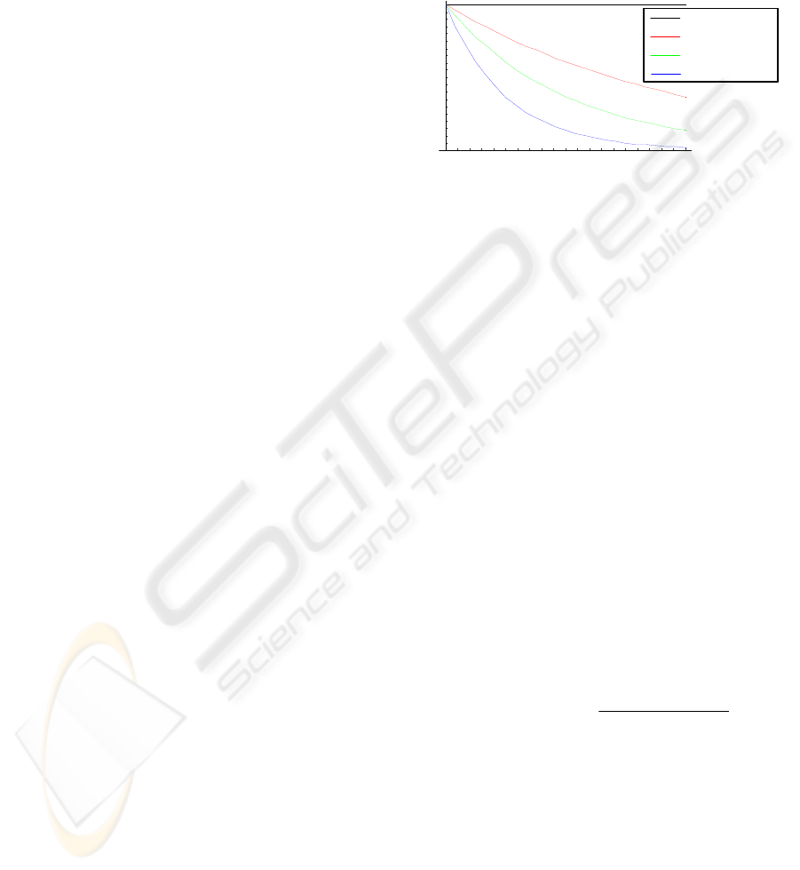
Based on this equation, we define the metric on

the layer of an attribute value. Thereby age(w, A)

denotes the age of the attribute value, which is cal-

culated by means of two factors: the point of time

when DQ is measured and the moment of data ac-

quisition. The decline rate decline(A) of attribute A’s

values can be determined statistically (see next sec-

tion). The metric on the layer of an attribute value is

therefore noted as:

),()(

:),(

AwageAdecline

Time

eAwQ

⋅−

(8)

Thereby Q

Time

(w, A) denotes the probability that

the attribute value is still valid. This interpretability

is an advantage compared to existing approaches.

Thereby the metric on the layer of an attribute value

(5) fulfils the requirements normalisation (R1) and

cardinality (R2). Figure 5 illustrates the results for

different parameters decline(A) depending on age(w,

A) graphically:

0.2

0.4

0.6

0.8

A)(w,Q

Time.

A)age(w,

0.75decline(A)

0.50decline(A)

0.25decline(A)

0.00decline(A)

0.2

0.4

0.6

0.8

A)(w,Q

Time.

A)age(w,

0.75decline(A)

0.50decline(A)

0.25decline(A)

0.00decline(A)

Figure 2: Value of the metric for selected values of decline

over time.

For attributes as e. g. “date of birth” or “place of

birth”, that never change, we choose decline(A) = 0

resulting in a value of the metric equal to 1:

Moreover, the metric is equal to 1 if an attribute

value is acquired at the moment of measuring DQ –

i. e. age(w, A) = 0:

The re-collection of an attribute value is also consid-

ered as an update of an existing attribute value.

1),(

0),(0),()(

====

⋅−⋅−

eeeAwQ

AwageAwageAdecline

Time

1),(

00)(),()(

====

⋅−⋅−

eeeAwQ

AdeclineAwageAdecline

Time

The metric on the layer of tupels is now devel-

oped based upon the metric on the layer of attribute

values. Assume T to be a tupel with attribute values

T.A

, T.A

,…, T.A

|A|

for the attributes A

, A

,…, A

|A|

Moreover, the relative importance of the attribute A

with regard to timeliness is weighted with

∈ [0; 1]. Consequently, the metric for timeliness

on the layer of tupels – based upon (8) – can be writ-

ten as:

∑

||21.

),.(

:),...,,,(

iiiTime

ATime

gAATQ

AAATQ

(9)

On the layer of relations and database the metric

can be defined referring to the metric on the layer of

attribute values similarly to the metric for consis-

tency (R4). The next section illustrates that the met-

rics are applicable in practice and meet the require-

ment adaptivity (R3).

ICSOFT 2007 - International Conference on Software and Data Technologies

5 APPLICATION OF THE

METRIC FOR TIMELINESS

The practical application took place within the cam-

paign management of a major German mobile ser-

vices provider. Existing DQ problems prohibited a

correct and individualised customer addressing in

mailing campaigns. This fact led to lower campaign

success rates.

Considering the campaign for a tariff option the

metric for timeliness was applied as follows: Firstly,

the relevant attributes and their relative importance

(R3) within the campaign had to be determined. In

the case of the mobile services provider’s campaign

the attributes “surname”, “first name”, “contact” and

“current tariff” got the related weights of 0.9, 0.2,

0.8 and 1.0. Hence the customer’s current tariff was

of great relevance, since the offered tariff option

could only be chosen by customers with particular

tariffs. In comparison the correctness of the first

name was less important. In the next step, the age of

each attribute had to be specified automatically from

the point of time when DQ was measured and the

moment of data acquisition. Afterwards, the value of

the metric for timeliness was calculated using de-

cline rates for the particular attributes that were de-

termined empirically or by means of statistics (see

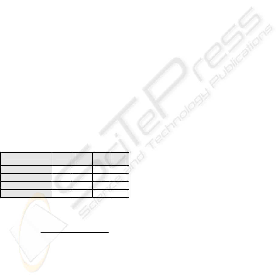
table 3 for an example).

Table 2: Determining timeliness by means of the devel-

oped metric (Example).

surname first

name

contact current

tariff

0.9 0.2 0.8 1.0

age(T.A

, A

) [year] 0.5 0.5 1.5 0.5

decline(A

) [1/year] 0.02 0.00 0.20 0.40

Time.

(T.A

, A

) 0.99 1.00 0.74 0.82

The value of the metric on the layer of tupels is

calculated via aggregation of the results on the level

of attribute values, considering the weights g

863.0

18.02.09.0

182.08.074.02.019.099.0

),...,,(

41.

≈

⋅

+⋅+

⋅

+⋅

=AATQ

Time

Hence the resulting value of the metric for timeli-

ness for the exemplary tupel is 86.3%, which means

that the tupel is for the given application (promoting

a tariff option) up to date at a level of 86.3%. The

mobile services provider used these results in its

campaign management. E. g. those customers (tupel)

with a result below 20% were sorted out and did not

receive any mailings. This is due to the fact that the

results of former campaigns showed the segment of

these customers being characterised by a success

rate close to 0. Applying the metrics improved the

efficiency of data quality measures and the measures

could be evaluated economically. E. g., only those

customer contact data with a value of the metric for

timeliness below 50% were brought up to date by

comparing these tupels to external data (e. g. to data

bought from German Postal Service). This reduced

the costs of acquiring addresses in a significant way.

In addition, the effects on the metric’s results and so

the improvements of the success rates of the cam-

paigns could be estimated. Thereby, the mobile ser-

vices provider was able to predict the measures’

benefits and compare them to the planned costs.

Besides these short examples for the metric’s ap-

plication resulting in both lower campaign’s and

measures costs, several DQ analyses were conducted

for raising benefits.

By applying the metrics, the mobile services

provider was able to establish a direct connection

between the results of measuring DQ and the suc-

cess rates of campaigns. Thereby the process for

selecting customers was improved significantly for

the campaigns of the mobile services provider, since

campaign costs could be cut down, too. Moreover,

the mobile services provider can take DQ measures

more efficiently and it can estimate the economic

benefit more accurately.

6 SUMMARY

The article analysed how DQ dimensions can be

quantified in a goal-oriented and economic manner.

The aim was to develop new metrics for the DQ

dimensions consistency and timeliness. The metrics

proposed allow an objective and automated meas-

urement. In cooperation with a major German mo-

bile services provider, the metrics were applied and

they proved appropriate for practical problems. In

contrast to existing approaches, the metrics were

designed according to important requirements like

interpretability or cardinality. They allow quantify-

ing DQ and represent thereby the foundation for

economic analyses. The effect of both input factors

on DQ – as e. g. decline over time – and DQ meas-

ures can be analysed by comparing the realised DQ

level (ex post) with the planned level (ex ante).

The authors are currently working on a model-

based approach for the economic planning of DQ

measures. For implementing such a model, adequate

DQ metrics and measurement procedures are neces-

sary. The approaches presented in this paper provide

a basis for those purposes. Nevertheless, further met-

rics for other DQ dimensions should be developed.

METRICS FOR MEASURING DATA QUALITY - Foundations for an Economic Data Quality Management

Besides, the enhancement of the metric for timeli-

ness in cases when the shelf-life can not be assumed

as exponentially distributed is a topic for further

research.

REFERENCES

Ballou, D. P., Wang, R. Y., Pazer, H., Tayi, G. K., 1998.

Modeling information manufacturing systems to de-

termine information product quality. In Management

Science, 44 (4), 462–484.

Campanella, J., 1999. Principles of quality cost, ASQ

Quality Press. Milwaukee, 3

edition.

Cappiello, C., Francalanci, Ch., Pernici, B., Plebani, P.,

Scannapieco, M., 2003. Data Quality Assurance in

Cooperative Information Systems: A multi-

dimensional Quality Certificate. In Catarci, T. (edi.):

International Workshop on Data Quality in Coopera-

tive Information Systems. Siena, 64-70.

English, L., 1999. Improving Data Warehouse and Busi-

ness Information Quality, Wiley. New York , 1

edi-

tion.

Eppler, M. J., 2003. Managing Information Quality,

Springer. Berlin, 2

edition.

Even, A., Shankaranarayanan, G., 2005. Value-Driven

Data Quality Assessment. In Proceedings of the 10th

International Conference on Information Quality.

Cambridge.

Feigenbaum, A. V. 1991. Total quality control, McGraw-

Hill Professional. New York, 4

edition.

The Data Warehousing Institute, 2002. Data Quality and

the Bottom Line: Achieving Business Success through

a Commitment to High Quality Data. Seattle.

Heinrich, B.; Helfert, H., 2003. Analyzing Data Quality

Investments in CRM – a model based approach. In

Proceedings of the 8th International Conference on

Information Quality. Cambridge.

Helfert, M., 2002. Proaktives Datenqualitätsmanagement

in Data-Warehouse-Systemen - Qualitätsplanung und

Qualitätslenkung, Buchholtz, Volkhard, u. Thorsten

Pöschel. Berlin 1

edition.

Hinrichs, H., 2002. Datenqualitätsmanagement in Data

Warehouse-Systemen, Dissertation der Universität

Oldenburg. Oldenburg 1

edition.

Jarke, M., Vassiliou, Y., 1997. Foundations of Data Ware-

house Quality – A Review of the DWQ Project. In

Proceedings of the 2nd International Conference on

Information Quality. Cambridge.

Juran, J. M., 2000. How to think about Quality. In Juran’s

Quality Handbook, McGraw-Hill. New York, 5

edi-

tion.

Lee, Y. W., Strong, D. M., Kahn, B. K., Wang, R. Y.,

2002. AIMQ: a methodology for information quality

assessment. In Information & Management, 40, 133-

146.

Machowski, F., Dale, B. G., 1998. Quality costing: An

examination of knowledge, attitudes, and perceptions.

In Quality Management Journal, 3 (5), 84-95.

Meta Group, 1999. Data Warehouse Scorecard. Meta

Group, 1999.

Redman, T. C., 1996. Data Quality for the Information

Age, Arctech House. Norwood, 1

edition.

Redman, T. C., 1998. The Impact of Poor Data Quality on

the Typical Enterprise. In Communications of the

ACM, 41 (2), 79-82.

SAS Institute, 2003. European firms suffer from loss of

profitability and low customer satisfaction caused by

poor data quality, Survey of the SAS Institute.

Shank, J. M.; Govindarajan, V., 1994. Measuring the cost

of quality: A strategic cost management perspective.

In Journal of Cost Management, 2 (8), 5-17.

Strong, D. M.Lee, Y. W., Wang R. Y., 1997. Data quality

in context. In Communications of the ACM, 40 (5),

103-110.

Wang, R.Y., Storey, V.C., Firth, C.P., 1995. A Framework

for analysis of data quality research. In IEEE Transac-

tion on Knowledge and Data Engineering, 7 (4),

623-640

White, D. J., 2006. Decision Theory, Aldine Transaction.

ICSOFT 2007 - International Conference on Software and Data Technologies