Weighted Evidence Accumulation Clustering

Using Subsampling

F. Jorge F. Duarte

, Ana L. N. Fred

, Fátima Rodrigues

João M. M. Duarte

and André Lourenço

GECAD – Knowledge Engineering and Decision Support Group

Instituto Superior de Engenharia do Porto, Instituto Superior Politécnico, Porto, Portugal

Instituto de Telecomunicações, Instituto Superior Técnico, Lisboa, Portugal

Abstract. We introduce an approach based on evidence accumulation (EAC)

for combining partitions in a clustering ensemble. EAC uses a voting mecha-

nism to produce a co-association matrix based on the pairwise associations ob-

tained from N partitions and where each partition has equal weight in the com-

bination process. By applying a clustering algorithm to this co-association ma-

trix we obtain the final data partition. In this paper we propose a clustering en-

semble combination approach that uses subsampling and that weights differ-

ently the partitions (WEACS). We use two ways of weighting each partition:

SWEACS, using a single validation index, and JWEACS, using a committee of

indices. We compare combination results with the EAC technique and the

HGPA, MCLA and CSPA methods by Strehl and Gosh using subsampling, and

conclude that the WEACS approaches generally obtain better results. As a

complementary step to the WEACS approach, we combine all the final data

partitions produced by the different variations of the method and use the Ward

Link algorithm to obtain the final data partition.

1 Introduction

Clustering is a procedure of partitioning data into groups or clusters based on a con-

cept of proximity or similarity between data. There is a huge amount of clustering

algorithms, even though no single algorithm can successfully discover by itself all

types of cluster shapes and structures. Recently, clustering ensemble approaches were

introduced [1-7,22-28] based on the idea of combining the partitions of a cluster en-

semble into a final data partition.

The concept underlying to EAC method, by Fred and Jain, is to combine the re-

sults of a cluster ensemble into a single combined final data partition, considering

each clustering result as an independent evidence of data organization. Using a voting

mechanism and taking the pairwise associations as votes, the N data partitions of n

patterns are mapped into an n

× n co-association matrix:

NvotesjiassocCo

/),(_ =

(1)

Jorge F. Duarte F., L. N. Fred A., Rodrigues F., M. M. Duarte J. and Lourenço A. (2006).

Weighted Evidence Accumulation Clustering Using Subsampling.

In 6th International Workshop on Pattern Recognition in Information Systems, pages 104-116

DOI: 10.5220/0002504501040116

 SciTePress

where votes

is the number of times the pattern pair (i,j) is assigned to the same clus-

ter among the N clusterings. The final data partition (P*) is obtained by applying a

clustering algorithm to the co-association matrix. The final number of clusters can be

fixed or automatically chosen using lifetime criteria [2,3].

Strehl and Ghosh explored graph theoretical concepts in the combination of clus-

tering ensembles. The partitions included in the clustering ensemble are mapped into

a hypergraph, where vertices correspond to samples, and partitions correspond to

hyperedges. They proposed three heuristics to try to answer the combination problem:

the hypergraph-partition algorithm (HGPA), the meta clustering algorithm (MCLA)

and the cluster-based similarity partitioning algorithm (CSPA).

Duarte et al. proposed the WEAC approach [4,5], also based on evidence accumu-

lation clustering. WEAC uses a weighted voting mechanism to integrate the partitions

of the clustering ensemble in a weighted co-association matrix. Two different meth-

ods are followed: SWEAC, where each clustering is evaluated by a relative or inter-

nal cluster validity index and the contribution of each clustering is weighted by the

value achieved for this index; JWEAC, where each clustering is evaluated by a set of

relative and internal cluster validity indices and the contribution of each clustering is

weighted by the overall results achieved with these indices. The final data partition is

obtained by applying a clustering algorithm to the weighted co-association matrix.

In this paper we test how subsampling techniques influence the combination re-

sults using the WEAC approach (WEAC with subsampling, WEACS). Partitions in

the ensemble are generated by clustering subsamples of the data set. Each subsample

has 80% of the elements of the data set. As with the WEAC approach, two different

methods are used to weight data partitions in the co-association matrix (w_co_assoc

matrix): Single Weighted EAC with subsampling (SWEACS) and Joint Weighted

EAC with subsampling (JWEACS).

We assessed experimentally the performance of the WEACS approach and com-

pared it with the single application of Single Link, Complete Link, Average Link, K-

means and Clarans algorithms and with the subsampling versions of EAC, HGPA,

MCLA and CSPA methods.

Section 2 summarize the cluster validity indices used in WEACS. Section 3 pre-

sents the Weighted Evidence Accumulation Clustering with subsampling (WEACS)

and the experimental setup used. In section 4 synthetic and real data sets are used to

assess the performance of WEACS. Finally, in section 5 we present the conclusions.

2 Cluster Validity Indices

Cluster validity indices address the following two important questions associated to

any clustering: how many clusters are present in the data; and how good the cluster-

ing itself is. For a summary of cluster validity measures and comparative studies see

for example [8,9] and the references therein.

We can use three approaches to do cluster validity [10]: external validity indices

assess the clustering results based on a structure that is assumed on the data set

(ground truth); internal validity indices assess the clustering results in terms of quanti-

ties that involve the vectors of the data set themselves; and relative validity indices

105

assess a clustering result by comparing it with other clustering results, obtained by the

same algorithm but with different input parameters.

In this work, we employed a set of widely used and referenced internal and relative

cluster validity indices, to evaluate the quality of the clusterings to be included and

weighted in the w_co_assoc matrix. We used two internal indices, the Hubert Statistic

and Normalized Hubert Statistic (NormHub) [11], and fourteen relative indices: Dunn

index [12], Davies-Bouldin index (DB) [13], Root-mean-square standard error

(RMSSDT) [14], R-squared index (RS) [14], the SD validity index [9], the S_Dbw

validity index [9], Caliski & Cooper cluster validity index [15], Silhouette statistic (S)

[16], index I [17], XB cluster validity index [18], Squared Error index (SE),

Krzanowski & Lai (KL) cluster validity index [19], Hartigan cluster validity index

(H) [20] and the Point Symmetry index (PS) [21].

3 Weighted Evidence Accumulation Clustering Using

Subsampling (WEACS)

The WEACS approach is an extension of the WEAC approach [4,5] by using sub-

sampling in the construction of the cluster ensemble. Both methods extend the EAC

technique by weighting differently data partitions in the combination process accord-

ing to cluster validity indices. The use of subsampling in WEACS has two main rea-

sons: to create diversity in the cluster ensemble and to test the robustness of the

method. In fact, other works have shown that the use of subsampling increase diver-

sity in the cluster ensemble leading to more robust solutions [22,24,26].

Like in WEAC, WEACS proposes the evaluation of the quality of each data parti-

tion by one or more cluster validity indices, which ultimately determines its weight in

the combination process. We can obtain poor clustering results in a simple voting

mechanism, if a set of poor clusterings overshadows another isolated good clustering.

By weighting the partitions in the weighted co-association matrix according to the

evaluation made by cluster validity and by assigning higher relevance to better parti-

tions in the clustering ensemble, we expect to achieve better combination results.

Considering n the number of patterns in a data set and given a clustering ensemble

{

}

PPP ,...,,

with N partitions of n*0.8 patterns produced by clustering sub-

samples of the data set, and a corresponding set of normalized indices with values in

the interval [0,1] measuring the quality of each of these partitions, the clustering en-

semble is mapped into a weighted co-association matrix:

w_co_assoc(i,j)=

(, )

Lij

vote VI

Si j

∑

(2)

where N is the number of clusterings, vote

Lij

is a binary value, 1 or 0, depending if the

object pair (i,j) has co-occurred in the same cluster (or not) in the L

partition,

the normalized cluster validity index value for the L

partition and (, )Si j is a matrix

such that (i,j)-th entry is equal to the number of data partitions from the total N data

partitions where both patterns i and j are simultaneous present. The final data partition

106

is obtained by applying a clustering algorithm to the weighted co-association matrix.

The proposed WEACS method is schematically described in table 1.

Table 1. WEACS approach.

Input:

n – number of data patterns of the data set

P =

{

}

PPP ,...,,

- Clustering Ensemble with N data partitions of n*0.8 patterns

produced by clustering subsamples of the data set

{

}

VIVIVIVI ,...,,

- Normalized Cluster Validity Index values of the corre-

sponding data partitions

Output: Final combined data partitioning.

Initialization: set w_co_assoc to a null n

n matrix.

1. For L=1 to N

Update the w_co_assoc: for each pattern pair (i,j) in the same cluster, set

w_co_assoc(i,j)=w_co_assoc(i,j)+

(, )

Lij

vote VI

Si j

vote

Lij

- binary value (1 or 0), depending if the object pair (i,j) has co-occurred in

the same cluster (or not) in the L

partition

- the normalized cluster validity index value for the L

partition

(, )Si j - number of data partitions where patterns i and j are present

2. Apply a clustering algorithm to the w_co_assoc matrix to obtain the final data

partition

In WEACS we used two different ways of weighting each data partition:

1. Single Weighted EAC with subsampling (SWEACS): in this method, the quality

of each data partition is evaluated by a single normalized relative or internal clus-

ter validity index, and each vote in the w_co_assoc matrix is weighted by the

value of this index:

VI =

(

)

norm validity P

(3)

2. Joint Weighted EAC with subsampling (JWEACS): in this method, the quality of

each data partition is evaluated by a set of relative and internal cluster validity in-

dices, and each vote in the w_co_assoc matrix being weighted by the overall con-

tributions of these indices:

VI =

(

)

NInd

ind

norm validity P

NInd

∑

(4)

where

NInd

is the number of cluster validity indices used, and

(

)

ind

norm validity P

is the value of the ind

validity index over the partition P

We used sixteen cluster validity indices in our experiments.

In the WEACS approach we can use different clustering ensembles construction

methods, different clustering methods to obtain the final data partition, and, particu-

107

larly in the SWEACS version, we can use even different cluster validity indices to

weight the data partitions. These constitute variations of the approach, taking each of

the possible modifications as a configuration parameter of the method. As shown in

the experimental results section, although the WEACS leads in general to good re-

sults, no individual configuration tested led consistently to better best results in all

data sets as compared to the subsampling versions of EAC, HGPA, MCLA and CSPA

methods. Strehl and Gosh [6] proposed to use the average normalized mutual infor-

mation (ANMI) as criteria for selecting among the results produced by different

strategies. The “best” solution is chosen as the one that has maximum average mutual

information with all individual partitions of the clustering ensemble. By comparing

the best results according to the consistency index with ground truth information (P

(Ci(P*,P

)), with the correspondent consensus values (ANMI) it was proved in [28]

and we could confirm in this work that there is no correlation between these two

measures; the mutual information based consensus function is therefore not suitable

for the selection of the best performing method.

To solve this problem we use a complementary step to the WEACS approach. It

consists in combining all the final data partitions obtained in the WEACS approach

with a clustering ensemble construction method or in combining of all the final data

partitions obtained in the WEACS approach with all clustering ensemble construction

methods. These data partitions are combined using the EAC approach and the final

data partition (P*) is obtained by applying a clustering algorithm to this new co-

association matrix.

3.1 Experimental Setup

3.1.1 Generation of Clustering Ensembles

There are several different approaches to produce clustering ensembles. We produced

clustering ensembles using a single algorithm (Single Link (SL), Complete-Link

(CL), Average-Link (AL), K-means and Clarans (CLR)) with different parameters

values and/or initializations, and using diverse clustering algorithms with diverse

parameters values and/or initializations. Specifically, each clustering algorithm makes

use of multiple values of k and K-means and Clarans in addition make use of multiple

initializations of clusters centers. We investigated also a clustering ensemble that

includes all the partitions generated by all the clusterings algorithms (ALL).

3.1.2 Normalization of Cluster Validity Indices

We can find two types of indices: some of them are intrinsically normalized and oth-

ers are not. In this work we use two indices intrinsically normalized and fourteen that

are not. The Normalized Hubert Statistic and Silhouette index are normalized be-

tween [-1,1] but we only consider values between [0,1].We use two internal validity

indices and fourteen relative validity indices. The best result for some indices is the

highest value and for others the lowest value. When the indices of the first type only

have values superior to zero, the normalization is made by dividing the value obtained

for the index by the maximum value obtained over all partitions (in-

dex_value=value_obtained/Maximum_value). When the indices of the second type

only have values superior to zero, the normalization is made by dividing the mini-

108

mum value obtained over all partitions by the partition value obtained for the index.

(index_value= Minimum_value/value_obtained). Some other indices increase (or

decrease) as the number of clusters increase and it is impossible to find neither the

maximum nor the minimum. With these indices, we look for the value of k where the

major local variation in the value of the index happens. This variation appears as a

“knee” in the plot and corresponds to the number of clusters existent in the data set.

The best value of this kind of indices typically is not the highest (or lowest) value

achieved. Thus, these indices can’t be incorporated directly in the w_co_assoc matrix.

The best value of these indices is where the “knee” appears. The value 1 is given to

the partition correspondent to the “knee” in the index. To incorporate these indices in

the co-association matrix we adopted the following approach: run the clustering algo-

rithms varying the number of clusters to be achieved between [1, k

maximum

] where

maximum

is the maximum number of clusters we suppose to exist in the data set; then,

we have to compare the partition correspondent to the “knee” with each of the other

partitions generated by this algorithm. We used an external index, the Consistency

index (C

), proposed in [1] to compare these clusterings. We utilized this approach to

Hubert Statistic, RMSSDT index, RS index and Squared Error index. The expected

number of clusters in Hartigan cluster validity index is the smallest k >=1 such that

H(k)<=10. Given that Hartigan index is not calculated for values of k greater than the

expected number of clusters (typically achieve negative values) we have to use to this

index the same procedure used to the indices based on the “knee” to achieve an index

value for partitions with k’s greater than the expected number of clusters. Table 2

shows the criteria to achieve the best value with each validity index.

Table 2. Criteria to obtain the best value according to each validity index.

Index Criteria Index Criteria Index Criteria Index Criteria

Hubert “Knee“ RMSSDT “Knee“ CH Max SE “Knee“

NormHub Max RS “Knee“ S Max KL Maximum

Dunn Max SD Min I Max H Smallest k:

H(k)<=10

DB Min S_Dbw Min XB Min PS Minimum

3.1.3 Extraction of the Final Combined Data Partition

The w_co_assoc matrix can be seen as a new similarity matrix between patterns; we

therefore apply a clustering algorithm to it to obtain the final combined data partition

P*. In our experiments, we assumed that the final number of clusters is known and

we used the k-means, SL, AL and Ward’s link (WR) algorithms to obtain the final

partition. To assess the performance of the combination methods, we compare the

final data partitions with ground truth information and we used the Consistency index

(Ci) to compare these partitions.

109

4 Experimental Results

4.1 Data Sets

Synthetic data sets For simplicity of visualization we considered 2-dimensional

patterns. These data sets were produced aiming the evaluation of the performance of

WEACS in a multiplicity of conditions, like distinct data sparseness in the feature

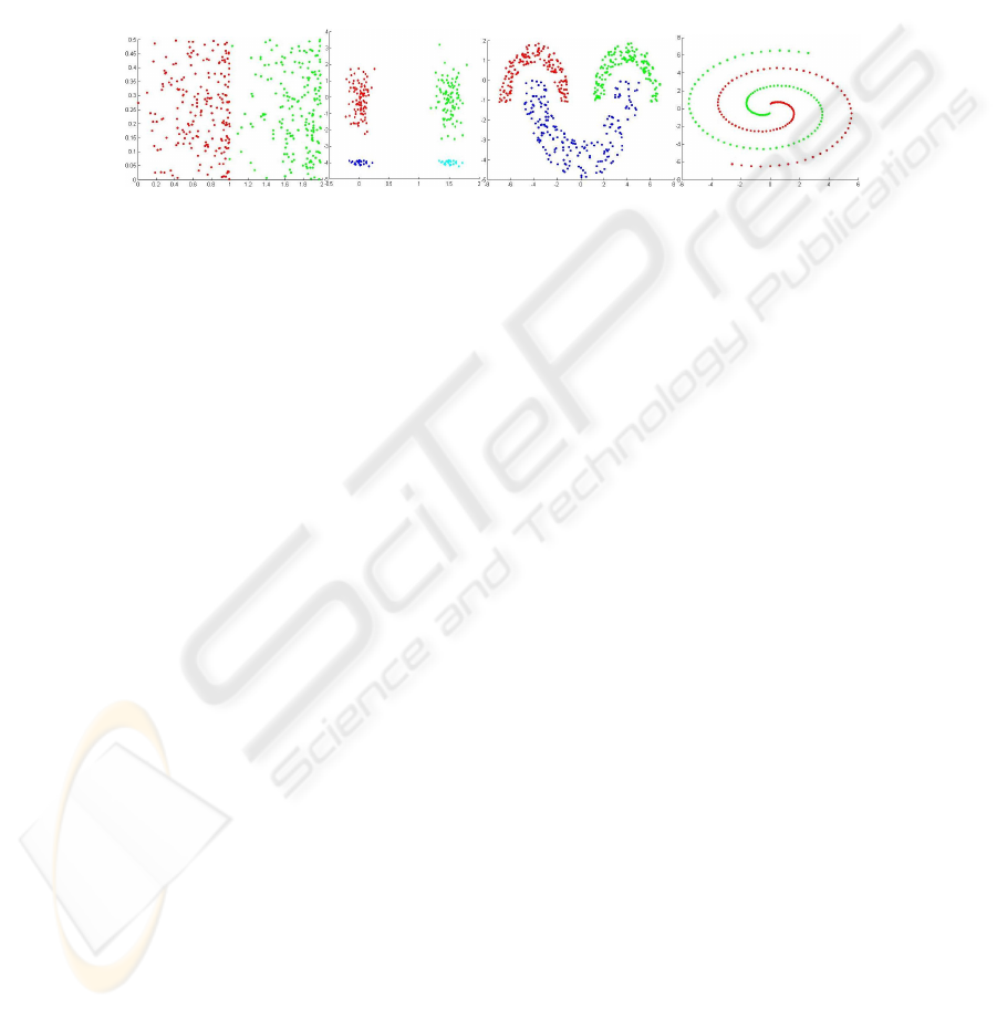
space, arbitrary shaped clusters, well separated and touching clusters. Figure 1 plots

these data sets.

(a) Bars (b) Cigar (c) Half Rings (e) Spiral

Fig. 1. Synthetic Data Sets.

The Bars data set has 2 classes (200 and 200) and the density of the patterns in-

creasing with increasing horizontal coordinate. The Cigar data set has 4 classes (100,

100, 25 and 25). The Half Rings data set is composed by 3 uniformly distributed

classes (150, 150 and 200) within half-ring envelops. The Spiral data set consists of

200 samples divided evenly in 2 classes.

Real Data Sets Four real-life data sets were considered to show the performance of

the WEACS: Breast Cancer, Iris, DNA microarrays and Handwritten Digits. The

Breast Cancer data set (http://www.ics.uci.edu/~mlearn/MLRepository.html) has 683

samples (9 features) spitted in two classes: Benign and Malignant. The Iris data set is

divided in three types of Iris plants (50 samples per class), characterized by 4 fea-

tures, and with one class well separated from the other two, which are intermingled.

The Yeast Cell data set (DNA microarrays) consists of the fluctuations of the gene

expression levels of over 6000 genes over two cell cycles. The available data set is

restricted to the 384 genes with 17 features (http://staff.washington.edu/kayee/model/)

whose expression level peak at different time points corresponding to the 5 phases of

the cell cycle. It was used the logarithm of the expression level (Log Yeast) and a

“standardized” version (Std Yeast) of the data (with mean 0 and variance 1). The

Handwritten Digits, is available at the UCI repository

(http://www.ics.uci.edu/~mlearn/MLRepository.html), and consists in 3823 samples,

each with 64 features. A subset (Optical) composed by the first 100 samples of all the

digits was used from a total of 3823 training samples (64 features).

4.2 Combination of Clustering Ensembles Using WEACS

The quality of the final data partition, P*, obtained with the WEACS method is

evaluated by calculating the consistency of P* with ground truth information P

110

using the Consistency index Ci(P*,P

). We assume that the true number of clusters is

known, being the number of clusters in P*.

Using subsamples of a data set (80% of the number of patterns in the data set), we

applied each of the clustering ensemble construction methods (SL, AL, CL, KM and

CLR) to generate 50 clustering ensembles each with 100 partitions with k randomly

chosen in the set {10,…,30}. Then, we applied the EAC, HGPA, MCLA, CSPA and

WEACS approaches to each of these clustering ensembles. Finally, we calculate the

average results over the 50 runs. Due to space limitations, it was not possible to pre-

sent results of the application of the subsampling version of EAC and WEACS ap-

proaches to all datasets. As an example, in table 3 we present C

(P*,P

) indices values

for SL, AL, CL, Clarans, K-means and ALL clustering ensembles with Std Yeast data

set. In this table, rows are grouped by the clustering ensembles construction method.

Inside each clustering ensemble construction method appears the four clustering

methods (K-means, SL, CL and WR) used to extract the final data partition. ALL

cluster ensemble construction method gather all the partitions produced by all the

methods (N=500).

Table 3. C

(P*,P

) indices values with Std Yeast data set.

EAC JWEACS Hubert Nhubert Dunn RMSSDT RS S_Dbw CH S index_I XB SE DB SD H KL PS

31.66 31.43 30.19 31.01 31.73 31.28 31.19 30.04 27.90 35.16 31.29 29.82 31.58 29.96 31.16 30.44 31.65 29.48

35.93 36.17 35.96 35.70 35.93 35.96 35.96 35.93 35.96 35.42 35.69 35.95 35.96 35.93 35.70 36.18 35.71 35.69

36.18 36.23 35.71 35.94 35.72 35.71 35.71 35.94 36.69 35.42 35.98 35.97 35.71 36.42 36.21 36.92 35.98 35.98

37.23 37.24 37.23 37.23 36.99 37.23 37.23 37.23 37.47 35.42 37.23 37.24 37.23 37.47 37.24 37.23 37.23 37.48

66.23 62.72 63.35 65.89 63.36 64.16 63.76 62.94 64.58 65.65 65.64 63.49 65.98 63.71 64.49 64.34 64.92 64.11

36.20 36.20 36.20 36.20 35.96 36.20 36.20 35.96 36.20 36.20 36.20 36.20 36.20 36.20 36.20 36.20 36.20 35.96

47.66 47.74 47.74 47.66 48.22 47.74 47.74 47.74 56.51 48.41 55.80 47.74 47.74 48.17 47.66 47.74 47.74 47.74

68.76 68.34 68.82 68.74 68.31 68.82 68.82 69.27 68.86 68.79 69.09 68.83 68.82 68.74 68.81 68.35 68.82 68.30

53.57 56.62 57.63 56.97 55.02 56.90 54.66 55.98 55.76 52.26 52.79 49.30 47.12 53.54 56.55 54.39 57.22 57.84

37.19 37.33 37.15 37.33 37.15 37.15 37.15 37.33 45.27 37.19 45.27 37.33 37.15 37.19 37.33 37.33 37.15 37.19

66.74 66.64 68.11 66.65 66.74 68.11 68.11 66.75 68.18 66.45 67.89 66.42 68.11 66.74 66.69 68.11 68.11 66.69

58.68 58.45 58.43 58.44 58.43 58.43 58.43 55.56 57.21 58.44 57.20 58.47 58.43 58.43 58.45 58.44 58.43 58.44

55.42 53.58 66.64 56.31 61.12 60.75 53.58 55.45 58.19 64.08 58.95 56.55 58.61 58.56 56.48 57.67 50.88 61.02

48.47 48.22 57.33 48.22 49.43 57.33 57.33 47.98 56.81 48.93 44.83 48.46 48.45 48.47 48.47 56.59 37.43 48.47

69.45 69.38 69.39 69.44 69.13 69.39 69.39 69.45 69.42 69.42 69.44 69.36 69.41 69.43 69.42 69.38 69.41 69.42

57.10 57.44 56.96 57.38 56.97 56.96 56.96 57.06 55.96 57.33 56.95 61.03 57.61 57.20 56.91 60.76 57.60 57.20

48.57 52.97 61.71 55.73 53.55 57.68 52.74 52.81 55.03 58.94 58.52 59.88 49.14 51.89 55.27 48.53 54.52 55.45

48.11 48.08 48.30 48.30 50.47 48.30 48.30 50.40 48.30 48.25 47.98 50.23 48.30 48.11 48.30 48.33 48.30 48.05

68.65 66.97 66.97 66.97 66.99 65.07 65.07 66.97 67.13 66.97 64.98 66.98 65.07 66.97 66.97 66.97 65.07 66.96

58.12 57.40 59.97 57.41 56.57 55.47 55.47 53.99 53.85 55.17 58.91 57.89 55.47 57.40 58.18 55.42 55.47 58.15

55.05 62.66 66.24 60.07 59.45 62.47 63.64 56.93 50.90 57.44 56.33 57.44 66.06 53.05 62.90 62.62 61.15 56.33

35.94 35.94 35.94 36.20 35.94 35.94 35.94 35.94 35.95 36.20 35.95 35.95 35.94 35.95 35.94 35.95 35.94 35.94

36.71 37.73 37.71 67.47 36.76 37.71 37.71 37.19 68.65 68.66 68.67 36.47 37.73 36.72 37.67 36.70 37.73 36.73

58.80

74.69

71.20 69.31 67.11 68.96 68.96 66.99 61.60

72.63

59.81 69.74 68.35 67.06 68.24 67.90 68.35 67.49

CLR

ALL

Comparing Ci results for the Std Yeast data set (table 3), we can see that both ver-

sions of the WEACS approach have a performance better than EAC. JWEACS ob-

tained 74,69% and SWEACS 72,63% in the best result over all cluster validity indi-

ces versus 69.45% of EAC. Analyzing the experimental results in the nine data sets,

we can see that none of the ensemble combination approaches systematically pro-

duces the best results in all the situations. However, in average, SWEACS and

JWEACS approaches produce better results when compared with EAC. The

JWEACS and the SWEACS results for each cluster validity index are in many situa-

tions equal to EAC results, in other situations the EAC results are improved with the

SWEACS and JWEACS approaches and in fewer situations the EAC results are bet-

ter than those of SWEACS and JWEACS.

By examining the clustering ensemble construction methods, we can observe that

in 6 of the 9 data sets used, the partitions of the ALL clustering ensemble construc-

tion method provide the best results in the EAC, JWEACS and SWEACS methods.

Therefore, we can say that the joint of all the partitions produced by all the clustering

ensemble construction methods is a good choice to construct cluster ensembles for

these approaches.

111

We obtained also results of the single application of each clustering algorithm (SL,

CL, AL, KM and CLR) to each data set. Table 4 presents best individual results pro-

duced by each clustering method (lines SL to KM) and best combined results per

combination strategy (lines EAC to Strehl) over 50 runs. In the 7

line of the table we

present the best Ci result of the 3 Strehl & Gosh heuristics (HGPA, MCLA and

CSPA).

Table 4. Ci results in SL, CL, AL algorithms and Ci best results in CLR, KM, Strehl, EAC and

WEACS approaches over 50 runs.

Spiral Log Yeast Std Yeast Optical Cigar Breast Iris Half Rings Bars

100 34.9 36.2 10.6 60.4 65.15 68 95 50.25

52 28.91 66.67 51.8 55.6 92.83 84 72 98.75

52 28.65 65.89 75.7 87.2 94.29 90.67 73.4 98.75

CLR

64.5 38.28 71.61 79.4 98 96.34 93.33 81.2 98.75

64.5 35.94 71.09 77.5 74.8 96.49 91.33 77.6 99.5

Strehl

100 37.94 65.57 84.98 72.81 96.48 98 95.05 99.5

EAC

100 40.93 69.45 82.73 100 97.07 93.95 100 99.5

SWEACS 100 41.58 72.63 84.31 100 97.2 93.33 100 99.5

JWEACS 100 41.51 74.69 82.39 100 97.07 93.33 100 99.5

Almost in all data sets the WEACS results outperform the single application of all

the clustering algorithms. In the Log Yeast and Std Yeast data sets, we can see the

superiority of the SWEACS and JWEACS approaches. In Cigar and Half Rings data

sets, both the EAC and WEACS approaches obtain 100%, which are much better

results than the ones obtained by other algorithms. The SWEACS approach obtained

in 4 data sets better best results than the EAC approach, in 5 data sets better best

results than the best result of the Strehl heuristics and in 3 data sets better best results

than the JWEACS version. On other hand, the EAC approach obtained only in 1 data

set a better best result than the SWEACS approach, in 2 data sets a better best result

than the JWEACS approach and in 5 data sets better best results than the best result

of the Strehl heuristics. Strehl heuristics obtained in 2 data sets better best results than

the EAC approach, in 2 data sets better best results than the SWEACS approach and

in 2 data sets better best results than the JWEACS approach. The JWEACS approach

obtained in 2 data sets better best results than the EAC approach, in 5 data sets better

best results than the best result of the Strehl heuristics and in 1 data set a better best

result than the SWEACS approach. The average percentage of improvement in the

best results of SWEACS as compared to EAC, over all data sets, was of 0,55% while

the average percentage of improvement in the best results of JWEACS as compared

to EAC, over all data sets, was of 0,54%. The average percentage of improvement in

the best results of SWEACS as compared to Strehl heuristics, over all data sets, was

of 4,25% while the average percentage of improvement in the best results of

JWEACS as compared to Strehl heuristics, over all data sets, was of 4,24%.

Table 5 shows the average Ci results of the CLR and KM algorithms and of the

combining clustering ensemble approaches over 50 runs. In the 4

line of the table we

present the average Ci result of the 3 Strehl & Gosh heuristics (HGPA, MCLA and

CSPA). We can see that none of the methods obtain in all data sets the best average

Ci results. The CLR and KM algorithms and the EAC and Strehl & Gosh approaches

112

obtain two best average Ci results and the JWEACS approach obtains one best aver-

age Ci result.

Table 5. Average Ci results of CLR, KM, Strehl, EAC and WEACS approaches over 50 runs.

Spiral Log Yeast Std Yeast Optical Ciga

Breast Iris Half Rings Bars

CLR

57.40 31.58 62.53 73.80 71.20 95.61 89.37 76.55 97.06

57.85 30.98 60.93 68.01 61.48 96.33 78.18 71.92 97.46

Strehl

68.37 32.25 51.59 69.44 68.11 80.03 93.72 93.04 96.04

EAC

71.78 34.78 50.68 58.55 83.23 77.32 70.38 84.98 83.19

SWEACS

70.97 34.37 51.96 57.23 82.13 77.55 71.84 83.24 80.71

JWEACS

70.83 34.62 51.67 57.60 83.63 77.37 70.76 84.86 83.24

Table 6 presents the C

results of all the final data partitions obtained after the ap-

plication of the complementary step to the WEACS approach.

Table 6. C

results of the final data partitions obtained after the applicaton of the complemen-

tary step to the WEACS approach.

Spiral Log Yeast Std Yeast Optical Cigar Breast Iris Half Rings Bars

KM 100.00 24.76 30.43 35.47 73.90 69.38 71.25 100.00 95.74

SL SL

100.00 34.94 35.95 11.60 94.98 65.15 65.36 100.00 95.75

AL 100.00 34.90 36.74 20.20 94.47 68.25 71.25 100.00 95.75

100.00 28.29 31.99 43.76 95.01 68.33 71.25 100.00 95.75

KM 50.51 33.99 65.88 73.26 80.37 96.78 77.27 100.00 64.25

AL SL 99.22 35.42 43.91 67.70 97.66 65.15 69.10 60.32 64.25

AL 50.98 35.42 63.32 67.29 98.20 65.15 69.10 99.60 64.25

WR 50.74 31.79 68.30 84.29 98.07 96.78 78.27 95.00 64.25

53.46 33.86 57.77 64.73 89.77 96.76 88.08 95.00 99.50

CL SL

96.40 30.21 67.86 60.42 99.58 95.35 74.67 95.00 67.78

50.94 29.82 58.89 72.19 99.58 96.61 74.67 95.00 99.50

WR 51.20 34.78 57.86 72.90 99.98 96.61 74.80 95.00 99.50

KM 51.03 36.97 56.82 72.82 63.79 67.94 88.12 88.18 98.67

KM SL 68.49 40.89 62.65 57.26 70.80 64.57 89.40 72.41 98.67

AL 51.77 40.89 69.42 79.49 70.80 67.92 89.53 82.91 98.67

51.81 40.89 55.16 78.08 70.80 67.94 89.53 99.23 98.67

98.27 35.26 54.44 64.65 71.32 90.58 80.39 92.59 98.75

CLR SL

97.82 36.39 57.14 39.19 100.00 69.75 52.00 99.80 96.68

79.96 34.81 67.10 78.55 100.00 69.65 52.00 93.64 98.75

WR 82.89 35.34 53.97 77.33 100.00 69.65 52.00 93.64 98.75

100.00 33.22 64.92 68.06 77.29 97.05 68.67 99.20 98.83

ALL SL

100.00 35.42 40.68 49.52 100.00 65.15 69.33 99.90 99.50

100.00 31.29 60.48 66.59 100.00 97.05 69.33 99.90 99.42

100.00 33.16 69.80 80.78 100.00 97.05 94.00 99.90 99.42

We can see in the last line of the table that by combining the final data partitions

obtained in the WEACS approach when it uses the partitions of the ALL clustering

ensemble construction method and then by applying the Ward Link algorithm

(ALL+WR) to obtain the final data partition we obtain in 5 (Spiral, Std Yeast, Cigar,

Breast Cancer and Iris data sets) of the 9 data sets the best Ci results and in 2 other

data sets (Half Rings and Bars) the results obtained are very close to the best Ci re-

sults. In the Half Rings data set, the result obtained is 99,90% while the maximum

obtained is 100% and in the Bars data set the result obtained is 99,42% while the

maximum obtained is 99,50%. In Optical data set the result obtained is 80,78%, a

value inferior to the maximum obtained by other combination, 84,29%. However, this

result (80,78%) is close to the maximum obtained by the EAC approach (82,73%)

and much superior to the average value obtained by the EAC approach (58,55%) and

113

all other combination clustering ensemble approaches. In Log Yeast data set the result

obtained is 33,16%, a value inferior to the maximum obtained by other combination,

40,89%. This result (33,16%) is inferior to the maximum obtained by the EAC

approach (40,93%) and a litle inferior to the average value obtained by the EAC

approach (34,78%) and by both versions of WEACS (34.37% and 34.62%).

However, this result (33,16%) is superior to the average value obtained by the CL

(28,91%), AL (28,65%), CLR (31,58%), KM (30,98%) and Strehl (32,25%) methods.

Table 7 presents the percentage difference (the improvement in the accuracy) be-

tween the performance of the WEACS approach with the complementary step

(ALL+WR) and the average values obtained with the single application of the algo-

rithms, EAC, WEACS and Strehl approaches in each data set. The last column shows

the average improvement relatively to each single algorithm and each combination

clustering ensemble approach by using the WEACS approach with the complemen-

tary step (ALL+WR), over all data sets. In all approaches this improvement is supe-

rior to 10%, allowing concluding that this approach is robust and that could be fol-

lowed to obtain good clusterings. It can also be seen that in all data sets, with the

exception of Std Yeast data set, the values obtained by the WEACS approach with the

complementary step (ALL+WR) obtain always better values than the average of all

the other approaches.

Table 7. Percentage difference (improvement) between the performance of the WEACS ap-

proach with the complementary step (ALL+WR) and the average values obtained with the

single application of the algorithms, Strehl, EAC and WEACS approaches in each data set.

Spiral Log Yeast Std Yeast Optical Cigar Breast Iris Half Rings Bars Improve

0.00 -1.74 33.60 70.18 39.60 31.90 26.00 4.90 49.17 28.18

48.00 4.25 3.13 28.98 44.40 4.22 10.00 27.90 0.67 19.06

48.00 4.51 3.91 5.08 12.80 2.76 3.33 26.50 0.67 11.95

CLR

42.60 1.58 7.27 6.98 28.80 1.44 4.63 23.35 2.36 13.22

42.15 2.18 8.87 12.77 38.52 0.72 15.82 27.98 1.96 16.77

Strehl

31.63 0.91 18.21 11.34 31.89 17.02 0.28 6.86 3.38 13.50

EAC

28.22 -1.62 19.12 22.23 16.77 19.73 23.62 14.92 16.23 17.69

SWEACS

29.03 -1.21 17.84 23.55 17.87 19.50 22.16 16.66 18.71 18.23

JWEACS

29.17 -1.46 18.13 23.18 16.37 19.68 23.24 15.04 16.18 17.72

5 Conclusions

In this paper we present the WEACS approach that explores the subsampling to in-

crease the diversity of the clustering ensembles and extends the idea of EAC, propos-

ing the weighting of multiple clusterings by internal and relative validity indices.

Partitions in the clustering ensembles are produced by clustering subsamples of the

data set using K-means, Clarans, SL, CL and AL algorithms. We make use of two

different techniques to combine the clustering ensembles: using only the partitions

generated by a single algorithm with different initializations and/or parameters val-

ues; and using partitions generated by different clustering algorithms with different

initializations and/or parameters values. Using a voting mechanism, the partitions of

the cluster ensembles are weighted in the SWEACS version by an internal or relative

index to be incorporated in a w_co_assoc matrix; in the JWEACS version all internal

and relative indices contribute to weight each partition. The combined data partition

114

is achieved by clustering the w_co_assoc matrix using the K-means, SL, CL, AL or

WR algorithms. Experimental results with both synthetic and real data show that

SWEACS lead in general to better best results than the EAC and Strehl methods.

However, no individual WEACS configuration leads systematically to the best results

in all data sets. As a complementary step to the WEACS approach we combine all the

final data partitions obtained by the use of the ALL clustering ensemble construction

method. We use the EAC approach to do this combination and we use the Ward Link

algorithm to obtain the final data partition. We reach almost in all data sets the best

results or values very close to the best results.

These results show that the association of the subsampling and the weighting

mechanisms with cluster combination techniques lead to good results.

References

1. A. Fred, “Finding consistent clusters in data partitions,”. in Multiple Classifier Systems,

Josef Kittler and Fabio Roli editors, vol. LNCS 2096, Springer, 2001, pp. 309-318.

2. Fred A., Jain A. K., “Evidence accumulation clustering based on the k-means algorithm,”

in S.S.S.P.R, T.Caelli et al., editor,., Vol. LNCS 2396, Springer-Verlag, 2002, pp. 442 –

451

3. Fred and A.K. Jain, “Combining Multiple Clusterings using Evidence Accumulation,”

IEEE Transactions on Pattern analysis and Machine Intelligence, Vol. 27, No.6, June 2005,

pp. 835-850.

4. F.Jorge Duarte, Ana L.N. Fred, André Lourenço and M. Fátima C. Rodrigues, “Weighting

Cluster Ensembles in Evidence Accumulation Clustering”, Workshop on Extraction of

Knowledge from Databases and Warehouses, EPIA 2005.

5. F.Jorge F.Duarte, Ana L.N. Fred, André Lourenço and M. Fátima C. Rodrigues, “Weighted

Evidence Accumulation Clustering”, Fourth Australasian Conference on Knowledge Dis-

covery and Data Mining 2005.

6. A. Strehl and J. Ghosh, “Cluster ensembles - a knowledge reuse framework for combining

multiple partitions,” Journal of Machine Learning Research 3, 2002.

7. B. Park and H. Kargupta, Data Mining Handbook, chapter: Distributed Data Mining. Law-

rence Erlbaum Associates, 2003.

8. M. Meila and D. Heckerman, “An Experimental Comparison of Several Clustering and

Initialization Methods”, Proc. 14th Conf. Uncertainty in Artificial Intelligence, p.p. 386-

395, 1998.

9. M. Halkidi, Y. Batistakis, M. Vazirgiannis, "Clustering algorithms and validity measures",

Tutorial paper in the proceedings of the SSDBM 2001 Conference.

10. Theodorodis, S., Koutroubas, K., Pattern Recognition. Academic Press, 1999.

11. Hubert L.J., Schultz J., “Quadratic assignment as a general data-analysis strategy,” British

Journal of Mathematical and Statistical Psychology, Vol.29, 1975, pp. 190-241.

12. Dunn, J.C., “Well separated clusters and optimal fuzzy partitions,” J. Cybern, Vol. 4, 1974,

pp. 95-104.

13. Davies, D.L., Bouldin, D.W., “A cluster separation measure,”. IEEE Transaction on Pattern

Analysis and Machine Intelligence, Vol. 1, No2, 1979.

14. S.C. Sharma, Applied Multivariate Techniques, John Willwy & Sons, 1996.

15. Calinski, R.B.& Harabasz, J, “A dendrite method for cluster analysis,” Communications in

statistics 3, 1974, pp.1-27.

16. Kaufman, L. & Roussesseeuw, P., Finding groups in data: an introduction to cluster analy-

sis, New York, Wiley, 1990.

115

17. U. Maulik and S. Bandyopadhyay, “Performance Evaluation of Some Clustering Algo-

rithms and Validity Indices,” IEEE Transactions on Pattern Analysis and Machine Intelli-

gence, Vol. 24, no. 12, 2002, pp. 1650-1654.

18. Xie, X.L., Beni, G., “A Validity Measure for Fuzzy Clustering,” IEEE Trans. Pattern

Analysis and Machine Intelligence, Vol. 13, 1991, pp. 841-847.

19. W. Krazanowski, Y. Lai, “A criterion for determining the number of groups in a dataset

using sum of squares clustering”, Biometrics, 1985, pp. 23-34.

20. J.A. Hartigan, “Statistical theory in clustering”, J. Classification, 1985, 63-76.

21. C.H. Chou, M.C. Su, E. Lai, “A new cluster validity measure and its application to image

compression”, Pattern Analysis and Applications, Vol. 7, 2004, pp. 205-220.

22. S.T. Hadjitodorov, L. I. Kuncheva, L. P. Todorova, Moderate Diversity for Better Cluster

Ensembles, Information Fusion, 2005, accepted

23. X. Z. Fern, C.E. Broadley, “Random projection for high dimensional data clustering: a

cluster ensemble approach”, 20th International Conference on Machine Learning,

ICML;Washington, DC, 2003, pp. 186-193.

24. S Monti; P. Tamayo; J. Mesirov; T. Golub, ”Consensus clustering: a resampling-based

method for class discovery and visualization of gene expression microarray data”, Machine

learning, 52, 2003, pp. 91-118.

25. A. Topchy, B. Minaei-Bidgoli, A.K. Jain, W. Punch, “Adaptive Clustering Ensembles”,

Proc. Intl. Conf on Pattern Recognition, ICPR’04, Cambridge, UK, 2004, pp. 272-275.

26. B. Minaei-Bidgoli, A. Topchy, W. Punch, “Ensembles of Partitions via Data Resampling”,

Proc. IEEE Intl. Conf. on Information Technology: Coding and Computing, ITCC04, vol.

2, April 2004, pp. 188-192.

27. E. Dimitriadou, A. Weingessel, K. Hornik, “Voting-Merging: An Ensemble Method for

Clustering”, Artificial Neural Networks – ICANN, August 2001.

28. Lourenço, A., Fred, “A. Comparison of Combination Methods using Spectral Clustering

Ensembles,” in Proc. Pattern Recognition on Information Systems, 2004.

116