Tracking and Prediction of Tumor Movement in the
Abdomen
Margrit Betke
1
, Jason Ruel
1
, Gregory C. Sharp
2
, Steve B. Jiang
2
, David P. Gierga
2
and George T. Y. Chen
2
1 Computer Science Department, Boston University, Boston, MA, USA
2 Department of Radiation Oncology, Massachusetts General Hospital, Boston, MA, USA
Abstract. Methods for tracking and prediction of abdominal tumor movement
under free breathing conditions are proposed. Tumor position is estimated by
tracking surgically implanted clips surrounding the tumor. The clips are seg-
mented from fluoroscopy videos taken during pre-radiotherapy simulation ses-
sions. After the clips have been tracked during an initial observation phase, mo-
tion models are computed and used to predict tumor position in subsequent frames.
Two methods are proposed and compared that use Fourier analysis to evaluate
the quasi-periodic tumor movements due to breathing. Results indicate that the
methods have the potential to estimate mobile tumor position to within a couple
of millimeters for precise delivery of radiation.
1 Introduction
The National Cancer Institute estimates that 8.9 million Americans have a history of
cancer in 1999 and more than 1,500 Americans die of cancer per day (Cancer Facts
and Figures 2005). In 2005, 253,500 new cases of cancer of the digestive system are
expected. The respective 5-year survival rates for cancer of the liver, pancreas, and
stomach are 8%, 4%, and 23%. Radiation therapy is an important treatment option that
can extend survival and relieve symptoms in many patients.
It is essential in radiation therapy to have accurate knowledge of the position and
volume of the tumor to effectively apply sufficient radiation to the tumor while min-
imizing exposure to the surrounding normal tissue. Treatment is commonly planned
in simulation sessions with fluoroscopy, an imaging method in which X-rays strike a
fluorescent plate that is coupled to a video monitor. Unfortunately fluoroscopy does
not provide a sufficient contrast between abdominal tumors and their surrounding soft
tissues, which have similar densities. In preparation of radiation therapy, radio-opaque
metal clips are therefore implanted around the tumor. The high-density clips can be
observed in the fluoroscopy video as they move with the tumor. The tumors change po-
sition and may deform due to various rigid and non-rigid body movements. Respiration,
in particular, causes significant internal movements of abdominal tumors. Gierga et al.
[12], for example, measured the average magnitude of peak-to-peak tumor motion for
seven patients to be 7.4 mm in the cranio-caudal and 3.8 mm in the anterior-posterior
direction.
Betke M., Ruel J., C. Sharp G., B. Jiang S., P. Gierga D. and George T. Y. Chen A. (2006).
Tracking and Prediction of Tumor Movement in the Abdomen.
In 6th International Workshop on Pattern Recognition in Information Systems, pages 27-37
DOI: 10.5220/0002471800270037
Copyright
c
 SciTePress

After the planning phase is over, radiation therapy is typically performed without
concurrent imaging of the tumor. Radiation sessions last several seconds to minutes
during which tumor motion is likely to occur. To prevent or reduce thoracic and ab-
dominal tumor movement, breath-hold and controlled breathing techniques have been
proposed [2, 21]. To compensate for tumor movements, respiratory-gating and motion-
adaptive radiotherapy have been introduced [14, 18,25]. The idea of the compensating
technologies is to operate the radiation beam depending on the tumor position. Gating
technology can be used to turn the radiation beam on or off whenever the tumor enters or
leaves the field of the beam, respectively. Tracking technology can be used to move the
radiation beam with the tumor. The SMART system [18] and the 4-D treatment system
[25] are two sample implementations of motion-adaptive radiotherapy techniques.
The appearance of the new technologies reinforces the need for image analysis
methods that can accurately determine tumor position in real time during the treatment
delivery process. For a method to be successful, it must work within the limitations im-
posed by (1) imaging, (2) computing, and (3) actuating processes: (1) The frame rate
of the imaging process directly impacts tracking accuracy, thus a high rate would be
desirable. However, when fluoroscopy is used as the imaging tool, patients are exposed
to radiation, and therefore a high frame rate cannot be employed. From the radiation
safety point of view, the tumor should be imaged as infrequently as possible. (2) For the
method to work in real time, the inverse of the frame rate limits the time the method can
take to capture a frame, measure tumor position in this frame, and accurately estimate
tumor position in subsequent frames. (3) The actuating process causes a latency prob-
lem – it takes time to move hardware components and control the radiation beam. The
unique frame-rate, processing-time, and latency issues distinguish the tumor tracking
problem from other motion estimation problems in computer vision, which typically
rely on high frame rates, do not have latency issues, and focus on estimating position
in the current frame based on measurements in previous frames, e.g., [8,9]. The two
methods proposed here address the latency problem by estimating the tumor position
for a large number of subsequent frames. Prediction accuracy is evaluated by varying
parameters such as length of the measurement period, sampling frequency during the
measurement period, and length of the prediction period.
The proposed methods model and predict a patient’s sinusoidal breathing patterns
based on Fourier analysis and least-squares fitting. Analysis of periodic motion can also
be found in the study of the cardiovascular system [1,3, 17] and in human gait analysis,
e.g., [6, 7,15,16]. Related fields are pattern matching of time series, e.g., [10, 19,20],
and data mining of periodic patterns, e.g., [13]. In radiation oncology, there has been
a relatively recent focus on tracking and prediction of tumor motion [5, 14, 18, 22, 24,
25]. Our work is bringing about a connection between these fields by introducing new
motion prediction algorithms and applying them to an urgent problem in radiotherapy.
Both methods have the potential to facilitate real-time tracking of the tumor motion
during the treatment process and allow for precise delivery of radiation dose to moving
abdominal tumors.
28

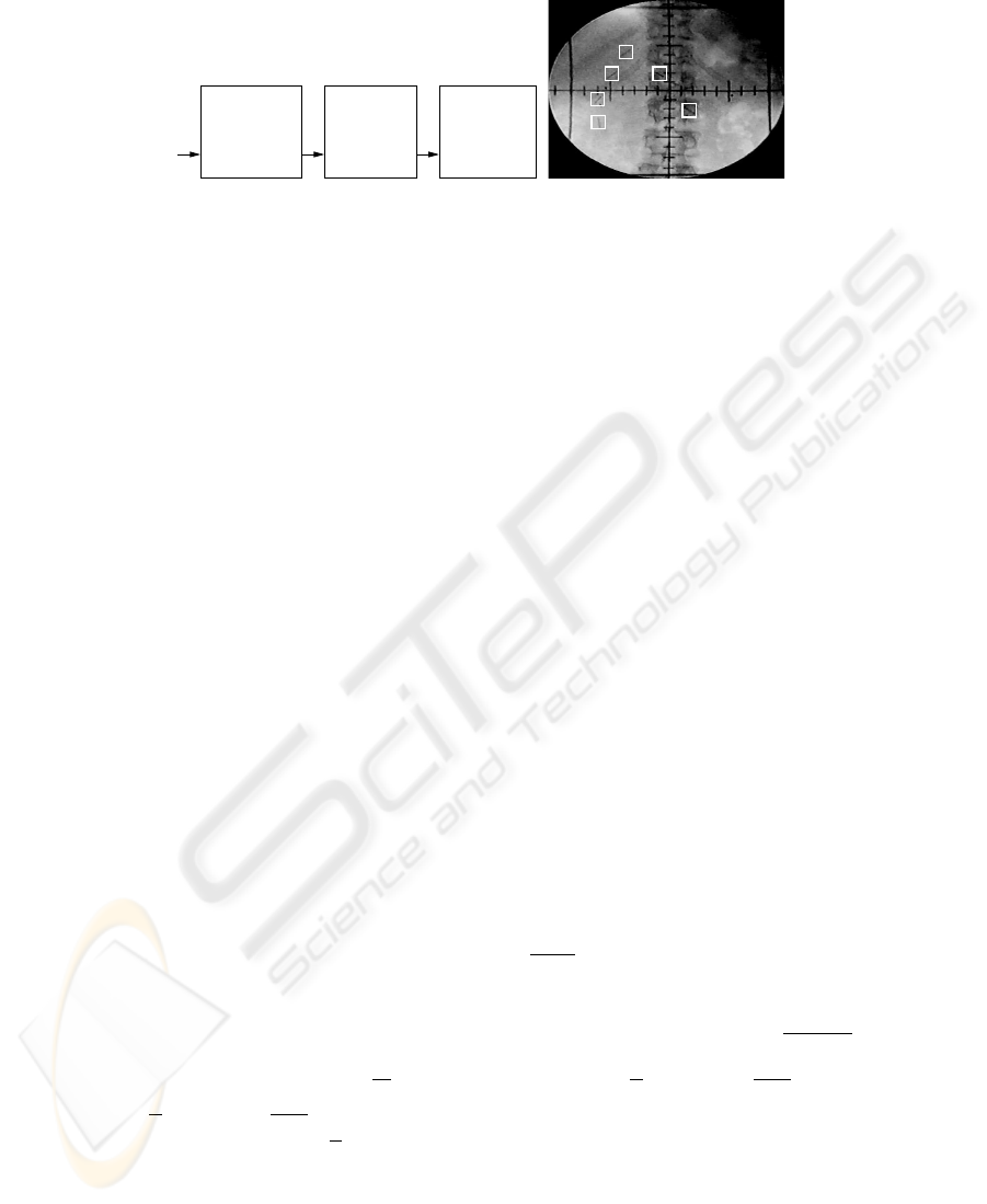
Clip Position
Tracking
Prediction
Motion
Frames
Motion
Modeling
FramesFramesFluoroscopy
Video 0, ..., k k−L +1, ..., k k+1, ..., k+L
PM
Fig.1. Left: Problem Overview. Right A fluoroscopy image of an abdominal tumor. The six clips
surrounding the tumor are marked by white squares.
2 Clip Tracking and Prediction Methods
An overview of the problem is given in Figure 1, left. The tracking process is performed
on each frame of the incoming fluoroscopy video stream. At current frame k, the clip
positions in the past L
M
image frames are used to model the tumor motion in the
modeling phase M . The model is then used to predict the tumor motion in the L
P
subsequent frames of prediction phase P . Tracking is initiated by manual selection of a
region containing the clip in the first frame of the fluoroscopy video, see Figure 1, right.
This region is further processed to isolate the clip from nearby clips that are potentially
included in the region. Each isolated clip is then matched and tracked in subsequent
frames using a template of a surgical clip. The template T is matched to the image I
by maximizing the normalized correlation coefficient. Tracking proceeds by finding
the subimage of each subsequent frame that best matches with the template. Breathing
is a quasi-periodic, roughly sinusoidal motion. The motion of internal organs due to
breathing is poorly understood. In the ideal case, the motion b(t) = (x(t), y(t), z(t))
T
of the abdominal tumor is due to regular breathing, i.e., periodic in T , so that b(t) =
b(t+T ) can be inferred from averaging the three-dimensional motion of its surrounding
clips. The motion can then be modeled with a simple sinusoidal waveform, for example,
b(t) = m + a cos(2πft − ψ), (1)
describing changes in position in the cranio-caudal direction with amplitude a, fre-
quency f = 1/T , phase ψ, and mean position m. With a more general, realistic model,
the breathing motion b(t) can be written as an infinite Fourier series
b(t) = m +
∞
X
n=1
a
n
cos

2πnt
T
− ψ
n

(2)
in “magnitude-angle form” [26], where T is the period of the signal b(t) = b(t +
T ), m = 1/T
R
T
t=0
b(t)dt is the mean or “DC” component of b(t), a
n
=
p
b
2
n
+ c
2
n
the magnitude, ψ
n
= arctan(
c
n
b
n
) the phase offset, b
n
=
2
T
R
T
0
b(t) cos
2π nt
T
dt and
c
n
=
2
T
R
T
0
b(t) sin
2π nt
T
dt. Equation 2 can also be written in terms of multiples of the
breathing frequency f
n
=
n
T
, which yields b(t) = m +
P
∞
n=1
a
n
cos (2πf
n
t − ψ
n
).
The cranio-caudal motion b(t) is measured at discrete points y[k] in time during
a finite window L
M
(see Section 2). If L
M
is chosen as an integral multiple of the
29

Predict Motion
m, a, f, ϕ
DFT
Tracker
Initial
No
Yes
Motion
Modeling
b(t) MSE
low ?
b(t)
Update
Clip Positions y[k]
S
S
Fig.2. Clip motion modeling using the shape function approach.
period T (at least approximately), the discrete-time sequence y[k] is periodic in L
M
with a discrete Fourier transform (DFT) Y [n] that is periodic in 1/L
M
. The transform
pairs are
y[k] =
L
M
−1
X
n=0
Y [n]e
j2πkn/L
M
and Y [n] =
1
L
M
L
M
−1
X
k=0
y[k]e
−j2πkn/L
M
. (3)
The power spectrum |Y [n]|
2
can be used to analyze the distribution of the frequency
coefficients of the data. If there is a strong peak in the power spectrum we may conclude
that there is a dominant frequency f
max
that models the breathing frequency well. This
frequency is the 1/T th frequency coefficient if L
M
is a multiple of T and nearby other-
wise. The dominant period T
max
is the inverse of f
max
. Analysis of the power spectrum
helps us determine whether an individual is breathing in a consistent pattern and also
whether there is a problem with the system such as jitter in the clip tracking process.
In the following sections we introduce two methods that use Fourier analysis to
characterize breathing motion. Both methods model the considerable variations in mean
m, amplitude a, and dominant frequency f of tumor motion that we and others, e.g.,
[18], have observed.
2.1 The Shape-function Approach
We developed a general motion model
b(t) = m + a S(Φ(t)), (4)
where the shape S is a quasi-sinusoidal function that maps a phase angle Φ(t) =
R
t
0
2πf(τ)dτ − ψ to a position in n-dimensional space, i.e., S : [0, 2π] → R
n
with
n = 1, 2 or 3. In our data, significant motion only occurs in the cranio-caudal direction,
so we present our waveform model and prediction algorithm for the case of n = 1. Our
approach, however, can also be generalized to model the two-dimensional motion of
clip position (x[k], y[k])
T
in fluoroscopy video. The approach also applies to 1D mea-
surements of air flow [5] and can be generalized to three-dimensional measurements
of the breathing motion obtained by the multiple x-ray imaging system described by
Shirato et al. [25].
The shape function S models the trajectory of the tumor over a single breathing
cycle. It is used as a waveform pattern or temporal template that models past move-
ments in order to predict future movements. Figure 2 shows the steps of the model-
ing process. To obtain the initial motion model b
1
(t), the parameters m
1
, f
1
, ψ
1
, and
30

a
1
are computed from the discrete Fourier transform of the first L
M
measurements
y[0], . . . , y[L
M
− 1] as described above.
The initial shape function S
1
is assumed to be a sinusoid from 0 to 2π. Accord-
ing to Equation 4, the first motion model is then b
1
(t) = m
1
+ a
1
sin(2πf
1
t − ψ
1
),
where the dominant frequency f
1
is chosen instead of the average frequency f
av
=
1/t
R
t
0
2πf(τ)dτ. The tumor positions predicted for future frames t + 1 to t + L
P
are
then b
1
(t + 1), . . . , b
1
(t + L
P
). To obtain a motion model b
k
(t) at time k, the previ-
ous shape function S
k−1
is used as S
k
, and the discrete Fourier transform of the last
L
M
position measurements y[k − L
M
+ 1], . . . , y[k] is computed, which yields the
parameters a
k
, f
k
, ψ
k
, and m
k
:
b
k
(t) = m
k
+ a
k
S
k
(2πf
k
t − ψ
k
). (5)
The mean squared error (MSE) between this model b
k
(t) and the measurements y[k −
L
M
+ 1], . . . , y[k] is computed to evaluate the accuracy of the model. If the error is too
large, the model is improved by updating the shape function as follows. The most recent
measured positions y[t] during a full period t = k − 1/f
k
+ 1, . . . , k are combined with
an appropriate discretization S
k
to yield
S
′
k
(Φ
k
(t)) = λw(t) S
k
(Φ
k
(t)) + (1 − λw(t)) y[t], (6)
where λ > 0.5 is a constant that gives the shape function more weight than the mea-
surements and w(t) is an exponential weighting function that gives recent measure-
ments greater weight than earlier measurements. The motion model b
k
(t) = m
k
+
a
k
S
′
k
(2πf
k
t − ψ
k
) is then used to predict the next L
P
tumor positions.
2.2 The Half-cycle Approach
The half-cycle approach is an alternative method for predicting abdominal tumor mo-
tion. Instead of using a shape function as a temporal template for one breathing cycle,
it uses a sinusoid as a template for half a breathing cycle. The approach computes a
sequence of sinusoids that models the motion history from the beginning of the video,
i.e., y[0], . . . , y[k], and is used to predict tumor positions y[k + 1], . . . , y[k + L
P
]. Each
sinusoid models the data during an inhalation or an exhalation phase.
We consider the mean m
k
of the data y[0], . . . , y[k] to be the “neutral” position of
a clip (or the collection of clips describing the tumor) that it assumes when inhalation
changes to exhalation and vice versa. The mean m
k
, dominant period T
k
, and phase
angle ψ
k
are obtained by Fourier analysis y[0], . . . , y[k] as described above. We then
subtract m
k
from the data so that the clip in the resulting sequence y
m
[0], . . . , y
m
[k] is
shifted to the ideal position 0 mm. Due to the digitization of time, the neutral position
typically occurs at zero crossings in the data. Not all zero crossings, however, corre-
spond to neutral positions because of noise in the measurements. We consider frame t
z
to contain a candidate zero crossing if either y
m
[t
z
] = 0 or if there is a sign change from
y
m
[t
z
−1] to y
m
[t
z
]. Phase ψ
k
is used to determine the first frame t
z
0
with a zero cross-
ing. The frame containing the next zero crossing is located in a small window around
t
z
0
+ T
k
/2. Subsequent zero crossings are found similarly by searching in a window
31

around the frame index obtained from adding the half of the dominant period to the
previous zero crossing. To select a single point among several candidate zero crossings
in the same window, we use a non-maximum suppression algorithm [23].
Once the zero crossings have been located, half a cycle of a cosine function is fitted
between each pair of crossings. The frequency of the jth cosine template is f
k,j
=
1/(2(t
z
j+1
− t
z
j
)), the phase is either
π
2
or
3π
2
, and the amplitude a
k,j
is computed
using a least squares method:
a
k,j
= arg min
a
t
z
j+1
−t
z
j
X
t=0
(a cos[2π(t + t
z
j
)f
k,j
− ψ
k,j
] − y
m
[t + t
z
j
])
2
. (7)
The parameters of the resulting j half-cycle cosine functions are then used as models to
predict the parameters of the j +1st half cycle. In particular, predicted frequency f
k,j+1
is the weighted average of the frequencies f
k,0
, . . . , f
k,j
. Each frequency is weighted
by its index so that the most recent breathing pattern is accounted for most. Predicted
amplitude a
k,j+1
is computed similarly from a
k,0
, . . . , a
k,j
. Predicted phase ψ
k,j+1
is
3π
2
if ψ
k,j
is
π
2
and
π
2
otherwise.
3 Results
The tracking and modeling methods were tested on fluoroscopy video of seven patients
obtained under clinical protocol during simulation sessions prior to radiation treatment.
The patient names used here are fictitious. The videos contained a total of 23 clips. We
verified by visual inspection that the clips were generally tracked reliably.
Radiation exposure time during the fluoroscopy sessions was limited to about seven
breathing cycles. The length of the videos ranged from 20 s to 36 s. For five sequences,
we were able to test our algorithm with a modeling window length of L
M
= 480,
which corresponded to about four breathing cycles. For the two shorter sequences, we
used L
M
= 380. We evaluated the prediction performance of the motion models for
the remaining breathing cycles. To obtain a sample that is sufficiently large for testing,
we moved the modeling window K = 100 times through the video, each time by one
frame. A length of L
P
= 10 was used for the prediction window.
Prediction accuracy of the motion model at time k is computed by averaging the
distances between predicted and eventually measured data points b(t) and y(t) over the
length of the prediction window: E(k) =
1
L
p
P
k+L
p
t=k
|b(t)−y(t)|. We also compute the
prediction accuracy of modeling the motion in a full video by averaging the results ob-
tained for the K motion models tested: E =
1
K
P
K
k=1
E
p
(k), where the first prediction
k = 1 starts at frame L
M
+ 1. The average errors for the seven patients was 1.64 mm
using the shape-function approach and 1.04 mm using the half-cycle approach, which
is considerably lower. However, the average variance in the error was 0.2 mm
2
for the
shape-function approach and 0.85 mm
2
for the half-cycle approach, which is consid-
erably higher. Table 1 shows the motion prediction results in more detail. Examples of
successful prediction using the two approaches are shown in Figure 3.
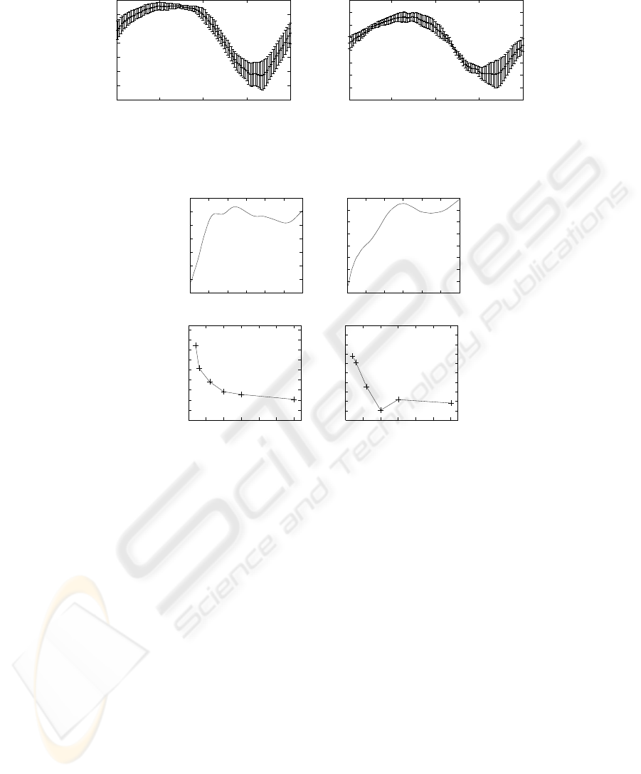
The average and standard deviations of the 100 shape functions are shown in Fig-
ure 4 for two patients. The graphs show the signal dependence of the standard deviation
32

Table 1. Prediction Results with the Shape-function Approach and the Half-cycle Approach.
Patient No. Prediction Error Period
of Average Variance in Hz
Clips in mm in mm
2
Shape Cycle Shape Cycle Shape Cycle
Alice 4 2.62 1.63 0.54 1.66 3.45 3.73
Bob 2 1.75 0.76 0.14 0.25 2.90 2.86
Carol 3 2.81 1.24 0.52 2.14 3.47 3.26
Doug 3 0.78 0.81 0.03 0.66 3.38 3.52
Eve 7 0.90 0.72 0.05 0.42 2.94 3.24
Frank 2 1.69 1.59 0.05 0.73 3.38 3.53
Gary 2 0.90 0.52 0.03 0.07 3.19 2.88
of the shape model. In particular, the position model deviates more for phase angles cor-
responding to inspiration than expiration. This indicates that our breathing prediction
in the direction of the cranium is more reliable than in the caudal direction.
The methods’ prediction accuracy over longer prediction windows was tested for
patient Eve. Eve’s video is the longest among the videos and allowed us to test K = 260
predictions. The error for the prediction window lengths L
P
= 1, . . . , 120 is shown in
Figure 5, top, for the two methods. We also evaluated the prediction accuracy of motion
models that were computed over modeling windows with the same length but sparser
sampling. Figure 5, bottom, shows the average prediction error when the output of the
tracker is sampled at a rate of 30/j Hz for j = 1, 2, . . . , 15. The average errors for
sampling rates 10 Hz, 15 Hz, and 30 Hz are approximately the same.
4 Discussion and Conclusions
We have introduced two motion modeling and prediction methods for tracking abdomi-
nal tumor movement. With average errors of 1.64 mm and 1.04 mm, the motion predic-
tion methods appear to model the tumor movement rather well. Our goal is to eventually
reduce the error to less than 1 mm in order to facilitate real-time tracking of the tumor
motion during the treatment process and allow for precise delivery of radiation dose to
mobile tumors.
In future work, we will examine whether a combination of the two approaches re-
sults in more accurate modeling and prediction performance. The zero-crossing analysis
in the half-cycle approach may serve to verify the frequency and phase estimation in the
shape function approach. Longer training times may improve prediction performance.
Longer sequences may be obtained without exposing patients to additional radiation by
tracking external markers that are placed on the patient’s abdomen with a visible-light
or infra-red video camera. Preliminary results [11] suggest that there is a correlation be-
tween the motion of the clips and such external markers. Our goal is to lower the frame
rate as much as possible to limit the imaging radiation dose delivered to the patient.
Our preliminary results indicate that a frame rate of 30 Hz may not be necessary for
reliable prediction of breathing motion. While both methods maintain low error rates
in the sampling experiment, more testing is needed to evaluate tracking performance at
reduced frame rates.
33

-8
-6
-4
-2
0
2
4
0 2 4 6 8 10 12 14 16 18 20
Bob: Position (mm)
Time (s)
-8
-6
-4
-2
0
2
4
0 2 4 6 8 10 12 14 16 18 20
Bob: Position (mm)
Time (s)
-5
-4
-3
-2
-1
0
1
2
3
4
0 5 10 15 20 25
Gary: Position (mm)
Time (s)
-5
-4
-3
-2
-1
0
1
2
3
4
0 5 10 15 20 25
Gary: Position (mm)
Time (s)
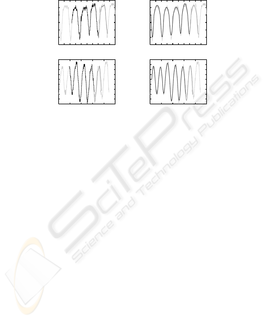
Fig.3. Position prediction results for Bob (top) and Gary (bottom) using the shape-function ap-
proach (left) and the half-cycle approach (right). The output from the tracker is shown in light
gray, the training period L
m
for the shape-function approach and the fitted sinusoids in the half-
cycle approach respectively in black, and the predicted positions in dark gray.
In addition to accuracy, ease of use is crucial for a new technology to become ap-
plicable to the clinical environment. With current technology, complete patient setup
and treatment in a busy clinic typically fit within a 15-minute appointment. Our al-
gorithms are therefore incorporated into an easy-to-use computer interface. A human
operator can use a single mouse click to select the image region that contains the clip in
the initial frame. The remaining tracking, modeling, and prediction processes are then
computed automatically.
For our future motion-adaptive radiotherapy system, we plan to use frame buffering
to store the images acquired while the operator selects the clips in the initial frame.
During this period, the patient keeps breathing and the clips move. The tracker must
analyze the buffered frames and then catch up to the incoming frames so that the clip
positions are tracked in real time.
Acknowledgements
Funding was provided by The Whitaker Foundation, the National Science Founda-
tion (IIS-0093367, P200A01031, and EIA-0202067), and the Office of Naval Research
(N000140110444).
34

-6
-5
-4
-3
-2
-1
0
1
π/2 π 3π/2 2π
Position (mm)
Phase (radians)
-5
-4
-3
-2
-1
0
1
2
3
π/2 π 3π/2 2π
Position (mm)
Phase (radians)
Fig.4. The average shape function and its standard deviation is computed over K = 100 models
for one of the clips of patient Bob (left) and of patient Doug (right).
0.75
0.8
0.85
0.9
0.95
1
1.05
1.1
0 20 40 60 80 100 120
Error (mm)
Prediction Window Length (Frames)
0.67
0.68
0.69
0.7
0.71
0.72
0.73
0.74
0.75
0 20 40 60 80 100 120
Error (mm)
Prediction Window Length (Frames)
0.45
0.5
0.55
0.6
0.65
0.7
0.75
0.8
0.85
0.9
0 5 10 15 20 25 30
Error (mm)
Sampling Rate (Hz)
0.4
0.42
0.44
0.46
0.48
0.5
0.52
0.54
0.56
0.58
0.6
0 5 10 15 20 25 30
Error (mm)
Sampling Rate (Hz)
Fig.5. Error in predicting tumor motion of patient Eve as a function of the length of the prediction
window L
P
(top) and sampling frequency (bottom) for the shape-function approach (left) and the
half-cycle approach (right).
References
1. Ashkenazy, Y, Ivanov, PC, Peng, SH CK, Goldberger, AL, and Stanley, HE (2001). Magni-
tude and sign correlations in heartbeat fluctuations. Phys Rev Lett, 86(9):1900–1903.
2. Balter, JM, Lam, KL, McGinn, CJ, Lawrence, TS, and Haken, RKT (1998). Improvement of
CT-based treatment planning models of abdominal targets using static exhalation imaging.
Int J Radiat Oncol Biol Phys, 41(4):939–943.
3. Bettermann, H, Cysarz, D, and Leeuwen, PV (2002). Comparison of two different ap-
proaches in the detection of intermittent cardioresperatory coordination during night sleep.
BMC Physiology, 4(2):1–18.
4. Cancer Facts and Figures 2005, American Cancer Society. http://www.cancer.org.
5. Chen, QS, Weinhous, MS, Deibel, FC, Ciezki, JP, and Macklis, RM (2001). Fluoroscopic
study of tumor motion due to breathing: facilitating precise radiation therapy for lung cancer
patients. Med Phys, 28(9):1850–1856.
35

6. Collins, RT, Gross, R, and Shi, J (2002). Silhouette-based human identification from body
shape and gait. In Proceedings of the 5th IEEE International Conference on Automatic Face
and Gesture Recognition, pages 366–371, Washington, DC.
7. Cutler, R and Davis, L S (2000). Robust periodic motion and motion symmetry detection.
In Proceedings of the IEEE Conference on Computer Vision and Pattern Recognition, pages
2615–2622, Hilton Head Island, SC.
8. Fagiani, C, Betke, M, and Gips, J (2002). Evaluation of tracking methods for human-
computer interaction. In Proceedings of the IEEE Workshop on Applications in Computer
Vision, pages 121–126, Orlando, FL.
9. Forsyth, DA and Ponce, J (2003). Computer Vision, A Modern Approach, pp. 373–398.
Prentice Hall, NJ.
10. Ge, X and Smyth, P (2000). Deformable Markov model templates for time-series pattern
matching. In Proceedings of the Sixth ACM SIGKDD International Conference on Knowl-
edge Discovery and Data Mining, pages 81–90, Boston, MA.
11. Gierga, DP, Chen, GTY, Kung, JH, Betke, M, Lombardi, J, Willett, CG (2004). Quantifica-
tion of respiration-induced abdominal tumor motion and its impact on IMRT dose distribu-
tions. Int J Radiat Oncol Biol Phys, 58(5):1584–1595.
12. Gierga, DP, Brewer, J, Sharp, GC, Betke, M, Willett, CG, Chen, GTY (2005). The correlation
between internal and external markers for abdominal tumors: implications for respiratory
gating. Int J Radiat Oncol Biol Phys, 61(5):1551–1558.
13. Indyk, P, Koudas, N, and Muthukrishnan, S (2000). Identifying representative trends in mas-
sive time series data sets using sketches. In Proceedings of the 26th International Conference
on Very Large Databases (VLDB’00), pages 363–372, Cairo, Egypt.
14. Keall, PJ, Kini, VR, Vedam, SS, and Mohan, R (2001). Motion adaptative x-ray therapy: a
feasibility study. Phys Med Biol, 46(1):1–10.
15. Lee, L and Grimson, WEL (2002). Gait analysis for recognition and classification. In Pro-
ceedings of the 5th IEEE International Conference on Automatic Face and Gesture Recog-
nition, pages 155–162, Washington, DC.
16. Little, JJ and Boyd, JE (1998). Recognizing people by their gait. Videre, 1(2):1–32.
17. Lotric, MB and Stefanovska, A (2000). Syncronization and modulation in the human car-
diorespiratory system. Physica A, 286:451–461.
18. Neicu, T, Shirato, H, Seppenwoolde, Y, and Jiang, SB (2003). Synchronized Moving Aper-
ture Radiation Therapy (SMART): Average tumor trajectory for lung patients. Phys Med
Biol, 48(5):587–598.
19. Noone, G and Howard, S (1995). Investigation of periodic time series using neural networks
with adaptive error thresholds. In Proceedings of the International Conference on Neural
Networks (ICNN), pages 1541–1545, Western Australia.
20. Oates, T, Firoiu, L, and Cohen, PR (1999). Clustering time series with hidden Markov
models and dynamic time warping. In IJCAI’99 Workshop on Neural, Symbolic, and Rein-
forcement Methods for Sequence Learning, 5 pages, Stockholm, Sweden.
21. Rosenzweig, KE, Hanley, J, Mah, D, Mageras, G, Hunt, M, Toner, S, Burman, C, Ling, CC,
Mychalczak, B, Fuks, Z, and Leibel, SA (2000). The deep inspiration breath-hold technique
in the treatment of inoperable non-small-cell lung cancer. Int J Radiat Oncol Biol Phys,
48(1):81–87.
22. Schweikard, A, Glosser, G, Bodduluri, M, Murphy, MJ, and Adler, JR (2000). Robotic
motion compensation for respiratory movement during radiosurgery. Comput Aided Surg,
5(4):263-277.
23. Shapiro, L G and Stockman, G C (2001). Computer Vision, page 299. Prentice Hall, NJ.
24. Shirato, H, Shimizu, S, Kitamura, K, Nishioka, T, Kagei, K, Hashimoto, S, Aoyama, H,
Kunieda, T, Shinohara, N, Dosaka-Akita, H, and Miyasaka, K (2000). Four-dimensional
36

treatment planning and fluoroscopic real-time tumor tracking radiotherapy for moving tumor.
Int J Radiat Oncol Biol Phys, 48(2):435–442.
25. Shirato, H, Shimizu, S, Kunieda, T, Kitamura, K, van Herk, M, Kagei, K, Nishioka, T,
Hashimoto, S, Fujita, K, Aoyama, H, Tsuchiya, K, Kudo, K, and Miyasaka, K (2000). Phys-
ical aspects of a real-time tumor-tracking system for gated radiotherapy. Int J Radiat Oncol
Biol Phys, 48(4):1187–1195.
26. Siebert, W (1986). Circuits, Signals, and Systems. MIT Press.
37