CPN BASED COMPONENT ADAPTATION
Yoshiyuki Shinkawa
Department of Media Informatics, Ryukoku University
1-5 Seta Oe-cho Yokotani, Otsu, Shiga, Japan
Keywords:
Component reuse, software engineering, colored Petri nets, formal methods.
Abstract:
One of the major activities in component based software development is to identify the adaptable components
to the given requirements. We usually compare requirement specifications with the component specifications,
in order to evaluate the equality between them. However, there could be several differences between those
specifications, e.g. granularity, expression forms, viewpoints, or the level of detail, which make the com-
ponent evaluation difficult. In addition, recent object oriented approaches require many kinds of models to
express software functionality, which make the comparison of the specification complicated. For rigorous
component evaluation, it is desirable to use concise and simple expression forms of specifications, which can
be used commonly between requirements and components. This paper presents a formal evaluation technique
for component adaptation. In order to relieve the granularity difference, the concept of a virtual component is
introduced, which is the reusable unit of this approach. A virtual component is a set of components that can
acts as single component. In order to express requirements and components commonly and rigorously, alge-
braic specification and Colored Petri Nets (CPNs) are used. Algebraic specification provides the theoretical
foundation of this technique, while CPNs help us to use it intuitively.
1 INTRODUCTION
One of the major tasks in Component Based Soft-
ware Development (CBSD) is to search and identify
the adaptable components to given requirements. For
this purpose, we usually compare the specifications
of requirements with those of components. There
have been proposed many theoretical and practicalap-
proaches to the component evaluation, which include
signature matching (Zaremski and Wing, 1993), spec-
ification matching (Zaremski and Wing, 1995), name
matching (Michail and Notkin, 1999), specification-
based browsing (Fischer, 1998), faceted classification
of software (Prieto-Diaz and Freeman, 1987), and
so on. When all the specifications are prepared in
the same manner, the above methods work correctly,
and help us to identify the adaptable components effi-
ciently.
However, in many cases, there would be several
kinds of gaps between the specifications of require-
ments and those of components, and the gaps make
the comparison complicated. The typical gaps that
we are often faced with are
1. A semantic gap, which is caused by the difference
in viewpoints between requirements and compo-
nents
2. A syntactic gap, which is caused by the difference
in notational rules
3. A structural gap, which is caused by the difference
in granularity
In addition to the above essential problems, there is
another notational problem to express specifications.
Since most specifications are expressed textually by
formal or informal languages, it is not so easy to un-
derstand the functionality that they intend to show. As
a result, the specification comparison becomes a dif-
ficult task. We need more visual notation tools as we
use in analysis and design phase, e.g. UML, DFD,
and IDEF.
This paper presents a formal approach to resolv-
ing the above mentioned gaps between requirements
and components, along with a visual notation method
for specifications. The paper is organized as follows.
In section 2, several formal approaches to resolving
the gaps are introduced. Section 3 shows how a tex-
tual notation of specifications is transformed into a
261
Shinkawa Y. (2006).
CPN BASED COMPONENT ADAPTATION.
In Proceedings of the Eighth International Conference on Enterprise Information Systems - ISAS, pages 261-268
DOI: 10.5220/0002456502610268
Copyright
c
 SciTePress

visual notation using Colored Petri Net (CPN). Sec-
tion 4 presents a process for identifying the adaptable
components to the given requirements using visually
expressed specifications.
2 RESOLVING GAPS BETWEEN
REQUIREMENTS AND
COMPONENTS
Before discussing component adaptability, we first
define what a component is. The word component
is often used vaguely in several contexts and situa-
tions. In CBSD, it usually means a unit of reuse,
however there are different kinds of units depending
on what programming environment we use. For ex-
ample, while procedural languages regard a subrou-
tine, a function, or a module as a unit of reuse, recent
object oriented languages regard a class as a unit of
reuse. The paper mainly focuses on the object ori-
ented programming environment, since it is one of the
most commonly used environments today, and reuse
is one of the most critical issues in it.
Roughly speaking, object orientation provides us
with two different ways for component reuse, that is,
class inheritance and method invocation. As a result,
there are two different units of reuse, namely a class
and a method. A class is a template of an object that
expresses encapsulated data and operations. The data
is implemented as a set of instance variables, and the
operations are implemented as a set of methods de-
fined in the class.
When we consider reusing an existing class
through inheritance, we have to decide whether each
method in the class is reused, overridden, or ig-
nored. In this decision, we evaluate the adaptability
of each method to a given requirement, and therefore
a method can be regarded as a unit of reuse even in
the class inheritance. Therefore, we treat a method
as a unit of reuse henceforth, and discuss how those
methods are reused.
The adaptability of a method is evaluated by com-
paring its specification with a requirement specifica-
tion. Those specifications have to be homogeneous
between requirements and components for rigorous
evaluation. However there could be several gaps be-
tween them.
2.1 Resolving a Semantic Gap
In order to create the specifications of requirements,
we first model the requirements from various view-
points. Since we focus on methods in classes for
reuse, function and behavior are the most essential
viewpoints for modeling. From a functional view-
point, a method acts as a data transducer which trans-
forms the arguments into the result value. On the
other hand, a method acts as a finite state machine
from a behavioral viewpoint, which responds to the
stimuli.
The specifications of components are also created
from either of the above two viewpoints. When a
requirement specification is compared with a com-
ponent specification for adaptability evaluation, both
the specifications have to be prepared from the same
viewpoint, unless we can not compare them eas-
ily. Consequently, all the requirement and component
specifications involved in the adaptability evaluation
must be prepared from the same viewpoint. If some
of the specifications have been prepared from the dif-
ferent viewpoint, there arises a gap between require-
ments and components.
Since those viewpoints give semantics to require-
ments and components, we refer to such gap as a se-
mantic gap. In order to resolve this gap, we first inves-
tigate the essential differences between function and
behavior.
A functional aspect of requirements and compo-
nents can be expressed by S-sorted functions in terms
of many sorted Σ algebra (Shinkawa and Matsumoto,
2000). Σ algebra provides an interpretation for the
signature Σ=(S, Ω), where S is a set of sorts, and Ω
is an S
∗
× S sorted set of operation names. S
∗
is the
set of finite sequences of elements of S.AΣ algebra
is an algebra (A, F ), where
1. A = {A
σ
|σ ∈ S} (a set of carriers) and
2. F = {f
A
|f ∈ Ω
σ
1
...σ
n
,σ
}
f
A
: A
σ
1
×···×A
σ
n
→ A
σ
(σ
1
,...,σ
n
,σ ∈ S).
When this f
A
map an element u
1
,...,u
n
 in the
domain of definition A
σ
1
×···A
σ
n
to an element v
in the co-domain A
σ
, we denote
f
A
(u
1
,...,u
n
)=v
S-sorted function f
A
is said to have arity σ
1
...σ
n
and result sort σ. The series of arity and result sort is
called the rank of the function.
If f
A
is a partial function, that is, if some elements
in the domain of definition A
σ
1
×···×A
σ
n
are not
mapped into the co-domain A
σ
, f
A
is denoted by
f : D (⊆ A
σ
1
×···×A
σ
n
) −→ A
σ
where D is a subset of the original domain of defini-
tion.
On the other hand, the behavioral aspect of a
requirement is expressed in many ways, e.g., Finite
State Machines (FSMs), Petri Nets, process algebra,
and so on. The behavioral aspect of a requirement
or a component expressed in the form of FSM is
represented as a sextuplet
Σ, Γ,S,s
0
,δ,ω where
ICEIS 2006 - INFORMATION SYSTEMS ANALYSIS AND SPECIFICATION
262

Σ is the input alphabet
Γ is the output alphabet
S is a finite non empty set of states
s
0
is an initial state
δ is the state transition function δ : S×Σ → S
ω is the output function ω : S × Σ → Γ
In order to reveal the essential difference between
function and behavior, we focus on the relationship of
inputs and outputs. When a requirement is given as an
S-sorted function, the inputs are transformed into the
output uniquely according to the mapping rule from
the domain to the co-domain.
On the other hand, when a requirement is given as
behavior, the output is determined by the output func-
tion ω : S × Σ → Γ, that is, the pair of a state and an
input determines the output. In addition, the state is
transferred according to the state transition function
δ : S × Σ → S. Therefore, the behavior is character-
ized by the function
β : S × Σ → S × Γ
Since the input to a software component is a set of
arguments, the output is a return value, and the state is
implemented as a set of instance variables, the above
function β is expressed as
β : A
σ
1
×···×A
σ
n
× B
ρ
1
×···×B
ρ
m
→ B
ρ
1
×···×B
ρ
m
× A
σ
where A
σ
i
s and A
σ
are the carriers of the arguments
and the result sort, and B
ρ
j
s are the carriers of the
instance variables.
If we regard the direct product
C = B
ρ
1
×···×B
ρ
m
× A
σ
as a co-domain, β is an S-sorted function
β : A
σ
1
×···×A
σ
n
× B
ρ
1
×···×B
ρ
m
→ C
This β implies that the behavioral aspect of a compo-
nent can be expressed as an S-sorted function. Simi-
larly, the behavioral aspect of a requirement can also
be expressed as an S-sorted function.
The above discussion leads us to create all the spec-
ifications in the form of S-sorted functions. We use
the term requirement function as a function that ex-
presses the requirement, and component function as a
function that expresses the component.
2.2 Resolving a Syntactic Gap
As discussed above, all the requirements and the com-
ponents can be treated as S-sorted functions. In order
to evaluate component adaptability to given require-
ments, we first have to express those functions in a
more concrete way. Roughly speaking, there are two
contrastive approaches to express those functions, or
more generally, objects or classes which include them
inside. One is the model-oriented approach that puts
emphasis on the structure of the object to be specified,
while the other is the property-oriented approach that
emphasizes the constraint on them (Fensel and Groen-
boom, 1995).
If a requirement specification and a component
specification are created by the different approaches,
we can not easily compare them for adaptability eval-
uation, and consequently all the related specifications
to be compared must be prepared by the same ap-
proach, that is, by either model or property oriented
approach. For component based software develop-
ment, the property oriented approach is more applica-
ble, since there might be no way to examine the struc-
ture of components.
In the property-oriented approach, the functional
aspect of requirements or components can be ex-
pressed by such algebraic specification languages as
OBJ (Goguen and Malcolm, 1996), CASL (Mosses,
1999), or Larch (Guttag and Horning, 1993). Even
though the syntax and semantics are different among
those languages, the basic structure of specifications
is almost the same. The specifications of require-
ments or components written in those languages con-
sist of two parts, often referred to as a signature part
and a axiom part.
A signature part defines the data types and opera-
tion names used in the specification, while an axiom
part describes the properties or the constraints that the
above operations must follow.
The axiom part consists of axioms which are ex-
pressed as equations of terms. A term is a formula
which can be derived from the signature of the speci-
fication. Terms are defined formally in the following
way.
1. An S-sorted variable x is a term
2. if t
1
,...,t
n
are terms, then f(t
1
,...,t
n
) is a term
An equation is a formula in the form of t = t

, where
t and t

are terms.
In addition to the functions defined in the signature
part, we assume the well-known functions to be used,
which include conditional branch function if-then-
else, projection function proj, tuple creation function
tuple, and so on. Those functions have the following
inherent properties.
proj(i, s)=s
i
tuple(s
1
,...,s
n
)=s
∀i [proj(i, s)=s
i
] ⇐⇒ s = tuple(s
1
,...,s
n
)
The function if-then-else is often denoted as
if t
1
then t
2
else t
2
where type(t
1
)=boolean , and type(t
2
)=
CPN BASED COMPONENT ADAPTATION
263

type(t
3
). Since
if-then-else(t
1
,t
2
,t
3
)=

t
2
(t
1
= true)
t
3
(t
1
= false)
and
f

if-then-else(t
1
,t
2
,t
3
)

=

f(t
2
)(t
1
= true)
f(t
3
)(t
1
= false)
holds, the if-then-else function has the property of
f

if-then-else(t
1
,t
2
,t
3
)

=
if-then-else

t
1
,f(t
2
),f(t
3
)

As an example, let us consider a bank account class
A with a method getBalance: A → int, and a method
debit: A × int → A. One of the axioms that the
methods must follow is
getBalance

debit(s, x)

= if-then-else

getBalance(s) − x ≥ 0, getBalance(s) − x,
getBalance(s)

where s ∈ A and x ∈ int.
The correctness of an equation of terms is proved
using the following inference rules, according to
equational calculus (?), where t, t

,t

and t
i
are
terms.
1. Reflexivity
t = t
2. Symmetry
t = t

t

= t
3. Transitivity
t = t

t

= t

t = t

4. Congruence
t
1
= t

1
, ··· ,t
n
= t

n
f(t
1
, ··· ,t
n
)=f(t

1
,...,t

n
)
2.3 Resolving Structural Gap
Even though we resolve the semantic and syntactic
gaps, there could be another gap between requirement
and component specifications. This gap occurs when
the granularity is different between them. Since the
granularity defines the structure of specifications, we
refer to such gap as a structural gap. In many cases,
this gap is resolved using glue codes to combine mul-
tiple components.
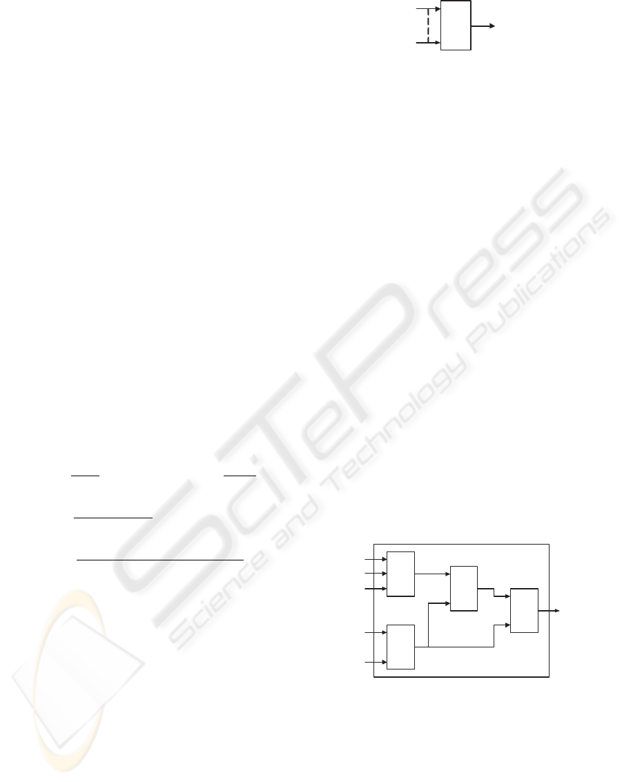
A component, or a method in our case, receives a
set of arguments to produce a return value. There-
fore, it can be depicted as a data transducer shown in
Figure 1. On the other hand, glue codes are placed be-
tween components to process the return values from
components, or to provide arguments to components.
A
x
1
x
2
y
Component
An output variable
with data types
Input variables
with data types
Figure 1: A component illustration.
Even though the use of glue codes can enhance the
components arbitrarily, it might reduce the productiv-
ity. In addition, the use of glue codes makes it diffi-
cult to evaluate the component adaptability to require-
ments, since glue codes can reconfigure component
based systems intentionally.
In order to make the component adaptability evalu-
ation precise, and make component usage simpler, we
consider combining components without glue codes.
Such combination of components is implemented by
connecting the output (or the return value) of a com-
ponent to the inputs (or the arguments) of other com-
ponents. Since arguments and return values are as-
sociated with data types, such connection is allowed
only when the data types of those outputs and inputs
match. For example, we obtain the combination of
components without glue shown in Figure 2, if data
types match between outputs and inputs. In Figure
2, x
i
and y
j
on the arrows represent the variables for
the arguments and the return values respectively. As-
suming type(x) shows the data type of the variable
x, type(x
6
)=type(y
1
), type(x
7
)=type(y
2
),
type(x
8
)=type(y
3
), and type(x
9
)=type(y
2
)
must hold.
A
B
C
D
x
1
x
2
x
3
x
4
x
5
y
y
1
y
2
x
6
x
7
y
3
x
8
x
9
Figure 2: A Virtual Component.
The component combination in Figure 3 can be re-
garded as a single component that receives a set of ar-
guments x
1
,x
2
,x
3
,x
5
,x
5
 and returns the value y.
We refer such combination of components as a virtual
component. A virtual component represents a compo-
nent based system without glue codes composed from
a set of available components. Therefore, a set of all
the possible virtual components shows the minimum
ICEIS 2006 - INFORMATION SYSTEMS ANALYSIS AND SPECIFICATION
264

adaptation capability of the available components. A
virtual component is formally defined as follows.
1. A virtual component receives multiple inputs and
yields a single output
2. Each input is associated with a data type and is con-
nected to at least one component in the virtual com-
ponent
3. Each input to a component in the virtual component
is either an input to the virtual component or an
output from another component
4. The output from the virtual component is associ-
ated with a data type, and is one of the output from
a component in virtual component
A single component is also a virtual component from
the above definition. A virtual component acts as a
single component, and therefore can be regarded as a
unit of reuse. Henceforth we use a virtual component
including a single component as a unit of reuse.
3 CPN BASED SPECIFICATIONS
Algebraic specifications can express requirements
and components accurately, however it seems diffi-
cult to understand them intuitively through text-based
specifications. As a software development methodol-
ogy, those specifications have to be expressed visu-
ally or graphically. UML is one of the most popular
graphical specification tools, however it is not suitable
to express the functionality of each method within
a class. Colored Petri Net is an alternative to UML
for expressing the functionality of a method within a
class.
CPNs are one of the enhancements of Petri nets,
and formally defined as follows (Jensen, 1997).
CPN=(S, P, T, A, N, C, G, E, I) ,
where
1. S : a finite set of non-empty types, called color sets
2. P : a finite set of places
3. T : a finite set of transitions,
4. A : finite set of arcs P ∩ T = P ∩ A = T ∩ A = ∅
5. N : node function A → P × T ∪ T × P
6. C : a color function P → S
7. G : a guard function T → expression
8. E : an arc expression function A → expression
9. I : an initialization function : P → closed expres-
sion.
In order to express the above discussed formal
specifications using CPN, we first define basic rela-
tionships between the elements of these two different
notations. As shown in the previous section, a formal
specification of a requirement or a component can be
denoted by
S
p
= Σ, {L
i
}
where Σ=S, Ω is a signature which is composed
of a set of sorts (data types) anf functions, and L
i
s are
the equations of terms that organize the axiom part
of the specification. A basic relationship between the
elements of such a specification and those of a CPN
is a s follows.
1. A function f
i
∈ Ω corresponds to a transition of a
CPN.
2. A variable x
j
of a function y = f
i
(x
1
,...,x
n
) cor-
responds to an input place of the transition associ-
ated with the function f
i
. A variable y corresponds
to an output place of that transition.
3. A color represents a data type or a sort. If a place
represents a variable x
j
∈ A
σ
j
, the color that is
associated with this place by the color function C
j
corresponds to the sort or the carrier A
σ
J
.
4. The if-then-else clause is implemented as a guard
function on a transition.
The above relationships map the signature Σ=
S, Ω to the transitions, the places, and the color sets
which compose the most basic elements in CPN. The
next step is to depict the axiom part {L
i
} in the form
of CPN.
Each L
i
is denoted by an equation t = t

where
t and t

are terms. A term is in the form of either
a variable or a function value f (t
1
,...,t
n
). A vari-
able x is depicted as a place, while a function value
f(t
1
,...,t
n
) is depicted by CPN iteratively as fol-
lows.
1. A function f is denoted by a transition with one
output place and multiple input places
2. Each argument t
i
is denoted by an input place to
the above transition. If t
i
is derived from another
function f

, that is, if t
i
= f

(t

1
,...,t

m
), the place
t
i
is an output place of the transition f

.
3. repeat the above process until all the input places to
the transitions become variables.
A CPN model constructed in the above way has
multiple places with no inbound arcs and one place
with no output arc. The former places represent the
initial inputs or arguments to the term that the CPN
model expresses, and the latter place represents the
final output or return value of the term. We refer to
the former places as initial input places and the lat-
ter place as final output place. The final output place
must have the only one transition that provides tokens
to it. This transition is called a terminal transition in
this paper.
Any term except single variable is expressed as a
CPN model of the above form. Such CPN model
CPN BASED COMPONENT ADAPTATION
265

is referred to as a functional CPN model in this pa-
per, since it represents data transformation that is per-
formed by the original term.
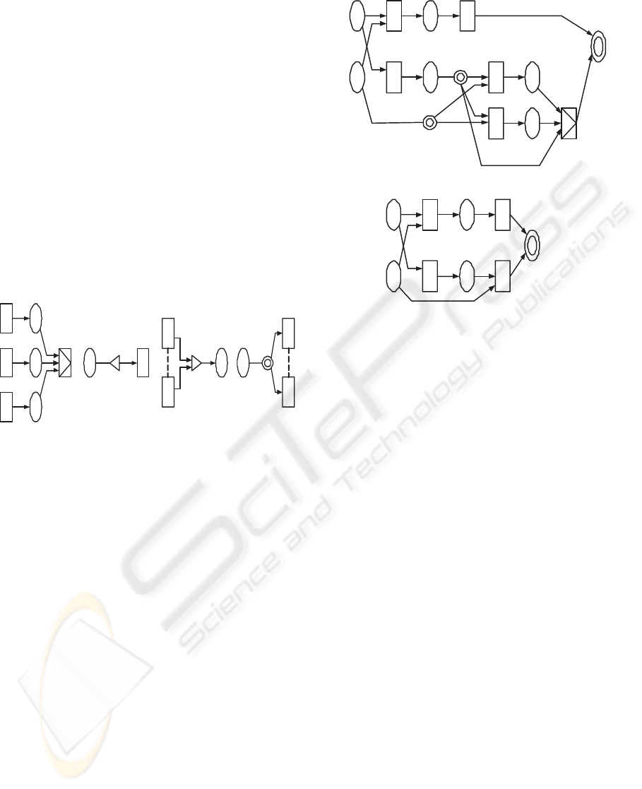
For notational convenience, we make a small en-
hancement to CPN models shown as follows. if-then-
else clause or function if-then-else(t1, t2, t3) is de-
noted as a rectangle with a triangle inside of it. ((a) in
Figure 3) A projection function proj which extracts
the ith element from a tuple, and tuple creation func-
tion tuple are denoted as figure (b) and figure (c) in
Figure 3 respectively. To create multiple copies of
a token, the distributor transition that is denoted by
a double lined circle shown as figure (d) in Figure 3
is used. We can depict a CPN models for an equa-
tion of terms without those enhancements. For ex-
ample, if-then-else transition can be substituted by
a guard function, however those enhancements make
CPN models simple, and reduce the size of the mod-
els.
i
(b). projection
(c). tuple creation
(d). distributor
t
1
t
2
t
3
(a). if-then-else
Figure 3: An enhancement to CPN models.
In order to express an equation of terms t = t

,
we introduce a new type of a place denoted by a dou-
ble lined ellipse, which is used as a common terminal
place of t and t

. For example, the debit method of a
bank account class A, which is expressed as a equa-
tion as discussed in the previous section
getBalance

debit(s, x)

=
if-then-else

getBalance(s) ≥ x,
getBalance(s) − x, getBalance(s)

and the credit method
getBalance

credit(s, x)

= getBalance(s)+x
are described as CPN models shown in Figure 4.
As shown above, an equation of terms is repre-
sented by two functional CPN models with common
initial input places and common single final output
place. Each functional CPN model may include other
functional CPN models inside. We refer to such inner
functional CPN models as subnets.
s
x
getBalance
minus
debit
gegetBalance
s
x
credit getBalance
getBalance plus
Figure 4: Example of CPN Models for Equations of Terms.
4 IDENTIFYING ADAPTABLE
COMPONENTS
Once all the requirement specifications and the com-
ponent specifications are transformed into CPN mod-
els, the next step is to identify an adaptable compo-
nent or a virtual component to a requirement. When
a component or a virtual component is adaptable to a
requirement, the function that represents the require-
ment in a requirement specification can be substituted
by the term that represents the component or the vir-
tual component. If all the requirement functions in a
requirement specification are substituted by the adapt-
able components or virtual components, the equations
of terms in the requirement specification are trans-
formed into the correct equations defined in the pre-
vious section.
In CPN models, a function is represented as a tran-
sition, and a term is represented as a subnet. Sub-
stitution of a requirement function by a component
is represented as replacement of a transition that ex-
presses the requirement function in the requirement
CPN model. When the substitution is done by a vir-
tual component, the transition is replaced by a subnet
that represents the virtual component. The simplest
form of CPN model that shows component adapta-
tion is shown in figure (a) in Figure 5, if the subnet
includes only component functions and well-known
functions. In this case, the upper shaded transition f
is implemented by the virtual component that is rep-
resented as the lower subnet. When the requirement
ICEIS 2006 - INFORMATION SYSTEMS ANALYSIS AND SPECIFICATION
266

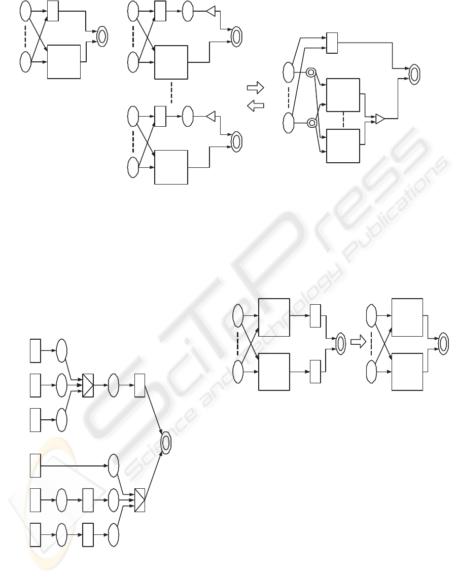
f
SN1
1
f
SNn
n
f
SN1
SNn
f
SN
(a). adaptation
(b). proj and tuple functions
SN : Subnet
Figure 5: Component Adaptation Rule – 1.
function yields a tuple as a return value, the adapta-
tion is represented by the figure (b) in Figure 5, from
the properties of proj and tuple functions.
In addition, the property of if-then-else function
introduced in the previous section is depicted as the
CPN model shown in Figure 6.
t
1
t
2
t
3
f
t
1
t
2
t
3
f
f
Figure 6: Component Adaptation Rule – 2.
However, most requirement CPN models have
much more complicated forms. In order to trans-
form the given requirement CPN model into the above
simple form, we introduce the reduction rule of CPN
models. The reduction rule is derived from the infer-
ence rule congruence in equational calculus discussed
in the previous section, and shown in Figure 7.
g
SN
SN’
g
SN
SN’
Figure 7: The Reduction Rule of CPN Models.
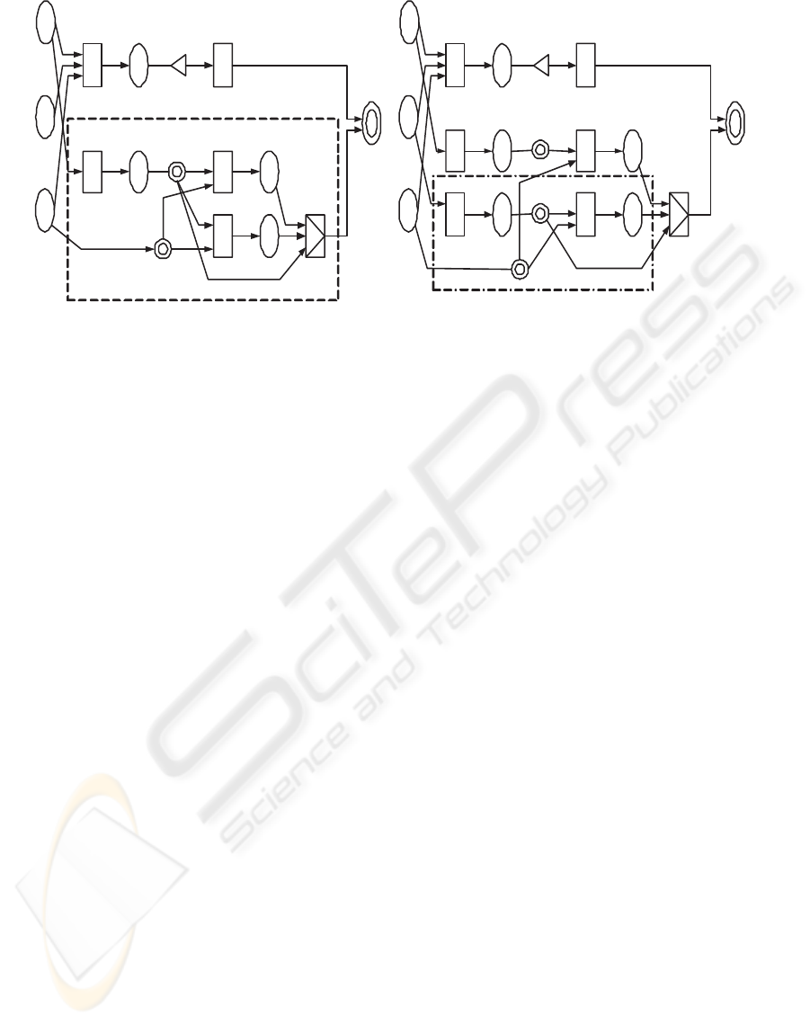
In order to show how the reduction process is used,
let us consider the transfer method
(a). getBalance

proj

1, transfer (s
1
,s
2
,x)


= if-then-else

getBalance(s
1
) − x ≥ 0,
getBalance(s
1
) − x, getBalance(s
1
))
(b). getBalance

proj

2, transfer (s
1
,s
2
,x)


= if-then-else

getBalance(s
1
) − x ≥ 0,
getBalance(s
2
)+x, getBalance(s
2
)

The CPN models of those equations are denoted as
shown in Figure 8. If we can use the methods get-
Balance, debit, and credit as components, that is, they
are implemented correctly, the CPN models in Fig-
ure 8 are reduced into the simple adaptation forms by
focusing on the subnets enclosed by the dotted lines,
CPN BASED COMPONENT ADAPTATION
267

s
1
s
2
x
1
getBalance
minus
ge
transfer
getBalance
s
1
s
2
x
2
getBalance ge
transfer
getBalance
getBalance
plus
Figure 8: CPN Models of the Method transfer.
and we can obtain the adaptable virtual component
transfer (s
1
,s
2
,x)=tuple

debit(s
1
,x),
if-then-else

getBalance(s
1
) − x ≥ 0,
credit(s
2
,x),s
2


5 CONCLUSION
A formal approach to identifying a set of compo-
nents which satisfies a single requirement was pre-
sented. In order to make component adaptability rig-
orous and simple, two different aspects of require-
ments and components, that is, function and behav-
ior are consolidated into a functional aspect. Such a
functional aspect is rigorously expressed in the form
of algebraic specifications, which consist of a set of
data type definitions and equations of terms. Those
terms are composed of S-sorted functions which rep-
resent basic requirements and components. When a
component satisfies a requirement function, the func-
tion that occurs in a requirement specification can be
substituted by the component function. In order to en-
hance the reusability of components, the concept of a
virtual component was introduced, which were com-
posed of multiple components, and acts as a single
component. Such a virtual component is expressed
as a term and the above substitution is based on this
term. As a software development methodology, we
need more visible and intuitive way to accomplish
the above substitution. A CPN model is one of the
most suitable solutions, since a CPN model can ex-
press terms and equations accurately, and the validity
of the substitution process can be implemented as a
reduction process of a CPN model.
REFERENCES
Fensel, D. and Groenboom, R. (1995). Formal specifica-
tion languages in knowledge and software engineer-
ing. In The Knowledge Engineering Review. 10(4)
pp.303-317.
Fischer, B. (1998). Specification-based browsing of soft-
ware component libraries. In Proc. of Thirteenth In-
ternational Conference on Automated Software Engi-
neering pp.74–83. ACM.
Goguen, J. A. and Malcolm, G. (1996). Algebraic Seman-
tics of Imperative Programs. MIT Press.
Guttag, J. V. and Horning, J. J. (1993). Larch: Languages
and Tools for Formal Specification. Springer.
Jensen, K. (1997). Coloured Petri Nets Volume 1-3.
Springer.
Michail, A. and Notkin, D. (1999). Assessing software li-
braries by browsing similar classes, functions and re-
lationships. In Proc. of International Conference on
Software Engineering, pp.463–472.
Mosses, P. D. (1999). Casl: A guided tour of its design. In
Proc. Workshop on Abstract Datatypes pp.216–240.
Prieto-Diaz, R. and Freeman, P. (1987). Classifying soft-
ware for reuse. In IEEE Software. 4(1) pp.6–16. IEEE.
Shinkawa, Y. and Matsumoto, M. J. (2000). Knowledge-
based software composition using rough set the-
ory. In IEICE Trans. on Inf. and Syst, Vol.E83-D.
No.4,pp.691-700. IEICE.
Zaremski, T. M. and Wing, J. M. (1993). Signature match-
ing: A key to reuse. In Proc. of the ACM SIGSOFT
’93 Symposium on the Foundations of Software Engi-
neering, pp182–190. ACM.
Zaremski, T. M. and Wing, J. M. (1995). Specification
matching of software components. In ACM Trans. on
Software Engineering and Methodology. 6(4), pp333–
369. ACM.
ICEIS 2006 - INFORMATION SYSTEMS ANALYSIS AND SPECIFICATION
268