BUSINESS PROCESS VISUALIZATION –

USE CASES, CHALLENGES, SOLUTIONS

∗

Stefanie Rinderle

, Ralph Bobrik

, Manfred Reichert

and Thomas Bauer

Dept. DBIS, University of Ulm, Germany

Information Systems Group, University of Twente, The Netherlands

DaimlerChrysler Research Center Ulm, Germany

Keywords: Business Processes Visualization.

Abstract: The proper visualization and monitoring of their (ongoing) business processes is crucial for any enterprise.

Thus a broad spectrum of processes has to be visualized ranging from simple, short–running processes to

complex long–running ones (consisting of up to hundreds of activities). In any case, users shall be able to

quickly understand the logic behind a process and to get a quick overview of related tasks. One practical

problem arises when different fragments of a business process are scattered over several systems where they

are often modeled using different process meta models (e.g., High–Level Petri Nets). The challenge is to ﬁnd

an integrated and user–friendly visualization for these business processes. In this paper we discover use cases

relevant in this context. Since existing graph layout approaches have focused on general graph drawing so

far we further develop a speciﬁc approach for layouting business process graphs. The work presented in this

paper is embedded within a larger project (Proviado) on the visualization of automotive processes.

1 INTRODUCTION

The proper visualization and monitoring of their (on-

going) business processes is crucial for anyenterprise.

Thus a broad spectrum of processes has to be visual-

ized ranging from simple, short-runningworkﬂows to

complex long-running processes (consisting of hun-

dreds of activities). In the automotive sector, for ex-

ample, this includes e-procurement and change man-

agement processes whereas the latter may be long-

running car engineering or release management pro-

cesses. In any case, users shall be able to quickly un-

derstand the logic behind a process and to get a quick

overview of their tasks. In practice, business process

data are often scattered over several application sys-

tems; i.e., a business process is splitted into differ-

ent more or less explicit fragments which are kept

and executed within different systems (Bobrik et al.,

2005). One consequence is that the deﬁnition and

control of these fragments are often based on different

process meta models

. One ﬁrst important challenge

∗

This work was conducted during a post doc stay at the

University of Twente which was fundend and supported by

DaimlerChrysler Research Ulm, Germany.

A meta model deﬁnes the constructs available for mod-

eling the process. Examples include Petri Nets, Activity

arising from the visualization of business processes

is to extract data about process fragments from the

different source systems and to provide an integrated

model of the overall process. Further if business pro-

cess data is completely available the challenge is to

ﬁnd a user-friendly layout of that process. Business

processes are often very complex as we have learned

from case studies in the automotive domain (Bobrik

et al., 2005). A typical process consists of dozens

up to hundreds of activities and comprises numerous

additional information (e.g., about process data ele-

ments, actors, and resources, cf. Fig. 2).

So far a lot of layout approaches for all kinds of

graphs (e.g., trees, DAGs, planar graphs, etc.) have

been presented in the literature (Eades et al., 1993;

Sugiyama, 2002). There are few approaches deal-

ing with the layout of business process graphs as well

(Fleischer and Hirsch, 2001; Kikusts and Rucevskis,

1995; Six and Tollis, 2002; Wittenburg and Weitz-

man, 1996a; Wittenburg and Weitzman, 1996b; Yang

et al., 2004). However, to our best knowledge, most

of them do not exploit the semantics of business pro-

cess graphs and only deal with graphs consisting of

untyped nodes and edges, i.e., graph nodes (edges)

cannot be distinguished. Fig. 1 depicts an example

Diagrams, and Statecharts.

204

Rinderle S., Bobrik R., Reichert M. and Bauer T. (2006).

BUSINESS PROCESS VISUALIZATION – USE CASES, CHALLENGES, SOLUTIONS.

In Proceedings of the Eighth International Conference on Enterprise Information Systems - ISAS, pages 204-211

DOI: 10.5220/0002452402040211

 SciTePress

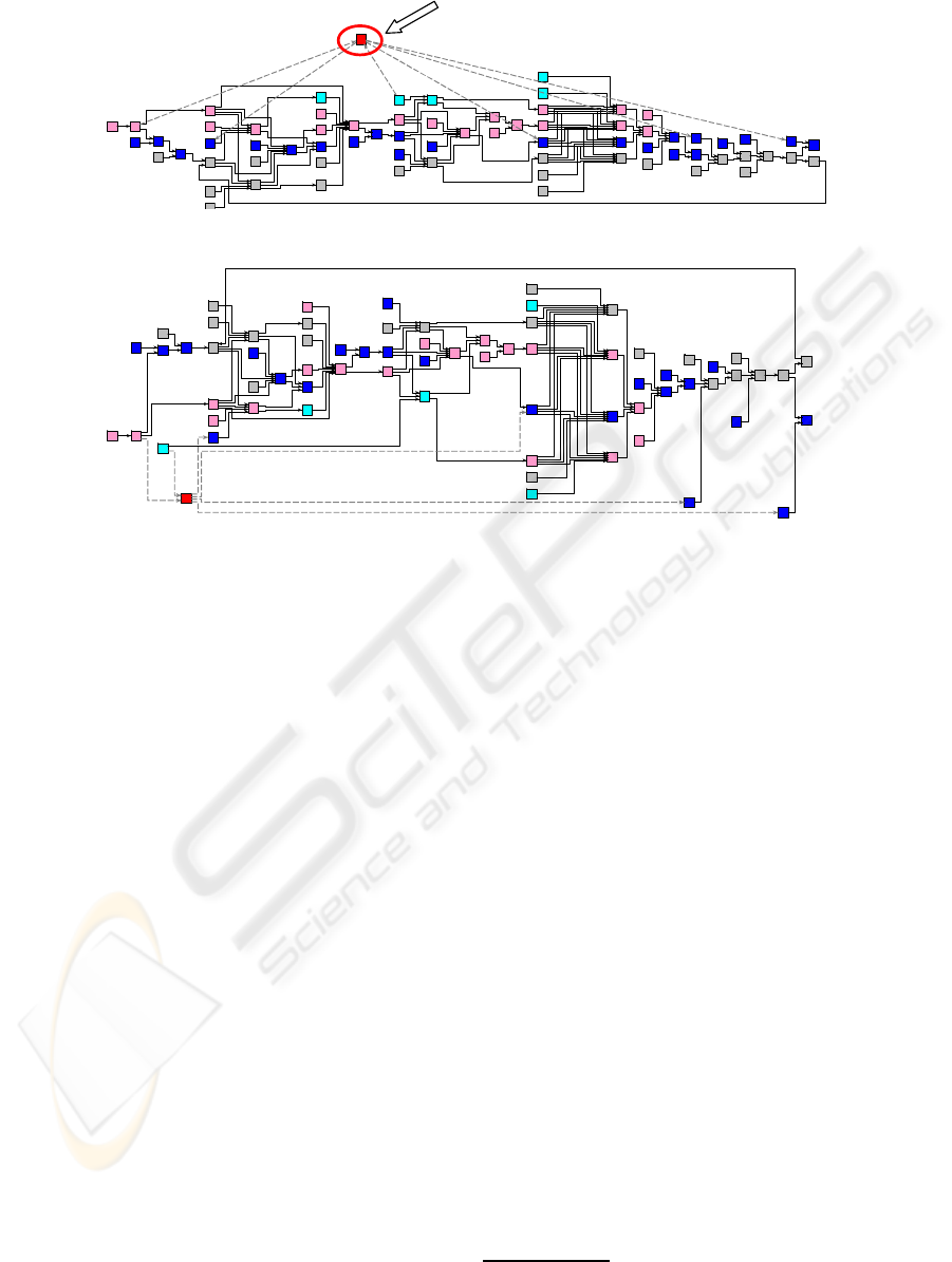
Figure 1: Change Management Process with Untyped Nodes and Edges.

for this case.

However, untyped nodes and edges do not reﬂect

the “nature” of business process graphs. Usually, re-

spective process graphs comprise nodes with (par-

tially) different semantics. This includes, for exam-

ple, nodes representing activities (i.e., process steps)

and nodes representing process data elements. Very

similar, edges of different type and semantics (e.g.,

control ﬂow and data ﬂow edges) have to be distin-

guished. Consider the process depicted in Fig. 2:

Activity nodes are represented as rectangles whereas

data element nodes are depicted as trapezoids. This

graphical distinction reﬂects the different roles these

elements possess with respect to the overall business

process. The challenge is to exploit such semantic in-

formation in order to build up an adequate layout for

business process graphs.

However, drawing business process graphs is not a

one-time task. In fact, the layout of business process

graphs is highly dynamic. As an example consider

the dynamic generation of business process views.

Such views on process graphs may vary from user

to user (Bobrik et al., 2005). Furthermore, especially

long-runningbusiness processes frequently have to be

changed due to several reasons (e.g., to adapt to new

laws or process optimizations) (Rinderle et al., 2004;

Reichert and Dadam, 1998). As a consequence the

process graph layouts have to be adapted accordingly.

In this context we need adequate approaches for re-

layouting business process graphs after changes. This

imposes several challenges including the provision of

automatic and efﬁcient algorithms for maintaining the

user’s “mental map” when a process change is per-

formed.

In this paper we summarize and describe several

use cases. We start with the layouting of business

processes graphs. Then we focus on relayouting busi-

ness process graphs after dynamic changes. Thereby

one goal is to maintain the user’s mental map of the

process. After this, we consider the visualization and

layouting of process instances (i.e., concrete business

cases created from a business process model). Fi-

nally, we shortly discuss how to display organiza-

tional structures of enterprises and end up with the

deﬁnition of certain

views

on business processes (e.g.,

only displaying the steps worked on by people of a

certain group).

Our approach exploits knowledge about the seman-

tics of graph nodes and edges in order to ﬁnd an ad-

equate process layout. We proceed in different steps

and allow users to specify which process constructs

shall be prioritized most when layouting a process

graph. As we know from our case studies, in most

cases, users want to start with layouting the control

ﬂow (i.e., the work tasks and the order in which they

are carried out). Therefore, we illustrate our approach

for layouting

control ﬂow skeletons

. In general, how-

ever, starting with the layouting of other process per-

spectives (e.g., data ﬂow) is conceivable as well. For

the control ﬂow layouts we impose several esthetic

criteria (e.g., mimizing the number of edge cross-

ings (Purchase, 2002)) which we meet by applying

a method based on preprocessing and permutation. In

order to complete the process graph layout additional

steps are discussed which show how to enhance the

control ﬂow skeleton layout with the other process el-

ements (e.g., process data elements or actors nodes).

In Section 2 we present use cases for visualizing

business process graphs. Related work is discussed in

Section 3. Section 4 presents our approach for lay-

outing business process graphs. We close with a sum-

mary and an outlook.

2 USE CASES

In order to come to a sophisticated approach for busi-

ness process graph visualization we ﬁrst have to con-

sider several use cases.

2.1 Business Process Graphs

The basis for business process visualization is to ﬁnd

an adequate approach for layouting process graphs.

As mentioned we may be confronted with process

fragments scattered over different information sys-

tems and being based on different process meta mod-

els. Actually an integrated and understandable visual-

ization of the whole business process is desired. In or-

der to achieve this we have to extract process knowl-

BUSINESS PROCESS VISUALIZATION - USE CASES, CHALLENGES, SOLUTIONS

205

Activity Actor Data Element

Control flow

edge

Synchronization

edge

Data flow

edge

Initiate change request Determine CR manager Instruct Expertise generate expertise (CAD)

generate expertise (car body)

generate expertise (motor)

generate expertise request evaluation

provide evaluation (plan)

provide evaluation (purchase)

provide evaluation (quality)

request comments

provide comments (plan)

provide comments (purchase)

provide comments (quality)

approve CR start realization (c) realize CR (construction) start realization(p)

conclude CR

CR initiator contact person CR manager

motor engineer

electronic engineer

car body engineer

development chief CR manager planning expert

purchase expert

quality expert

CR manager

ality expert

planning expert

purchase expert

CR approval board CR manager construction engineer CR manager

realize CR (production)

production engineer CR manager

change request

expertise (car body)

expertise (electronic)

expertise (motor)

expertise

evaluation (planning)

evaluation (purchase)

evaluation (quality)

evaluation

Figure 2: Change Management Process with Typed Nodes and Edges (Simpliﬁed).

edge from different logﬁles and application systems

and must then transfer the obtained process fragments

into the notion of a canonical process meta model.

Doing so one has to preserve potentially existing pro-

cess meta model properties (e.g., information about

the structuring of related process models) and exist-

ing layout information. This step is then followed by

layouting the whole business process using the graph-

ical notion of the canonical meta model. Thereby the

challenges are to (1) ﬁnd an algorithm for layouting

business processes graphs, (2) exploit the particular

semantics of the different process elements, and (3)

use available meta model properties and already ex-

isting layout information in order to optimize the pro-

cess layout algorithm

2.2 Dynamic Changes

Business processes change over time (e.g., by

adding/deleting process steps or dependencies be-

tween them) (Rinderle et al., 2004; Reichert and

Dadam, 1998). There are several approaches sup-

porting such changes (Rinderle et al., 2004). When

changing the structure (or logic) of a business process

it is important that this is also reﬂected by adapting

the layout of the business process graph accordingly.

The challenge is to avoid that users lose their

mental

map

when changing the process. Note that this could

be the case if we relayout the process “from scratch”

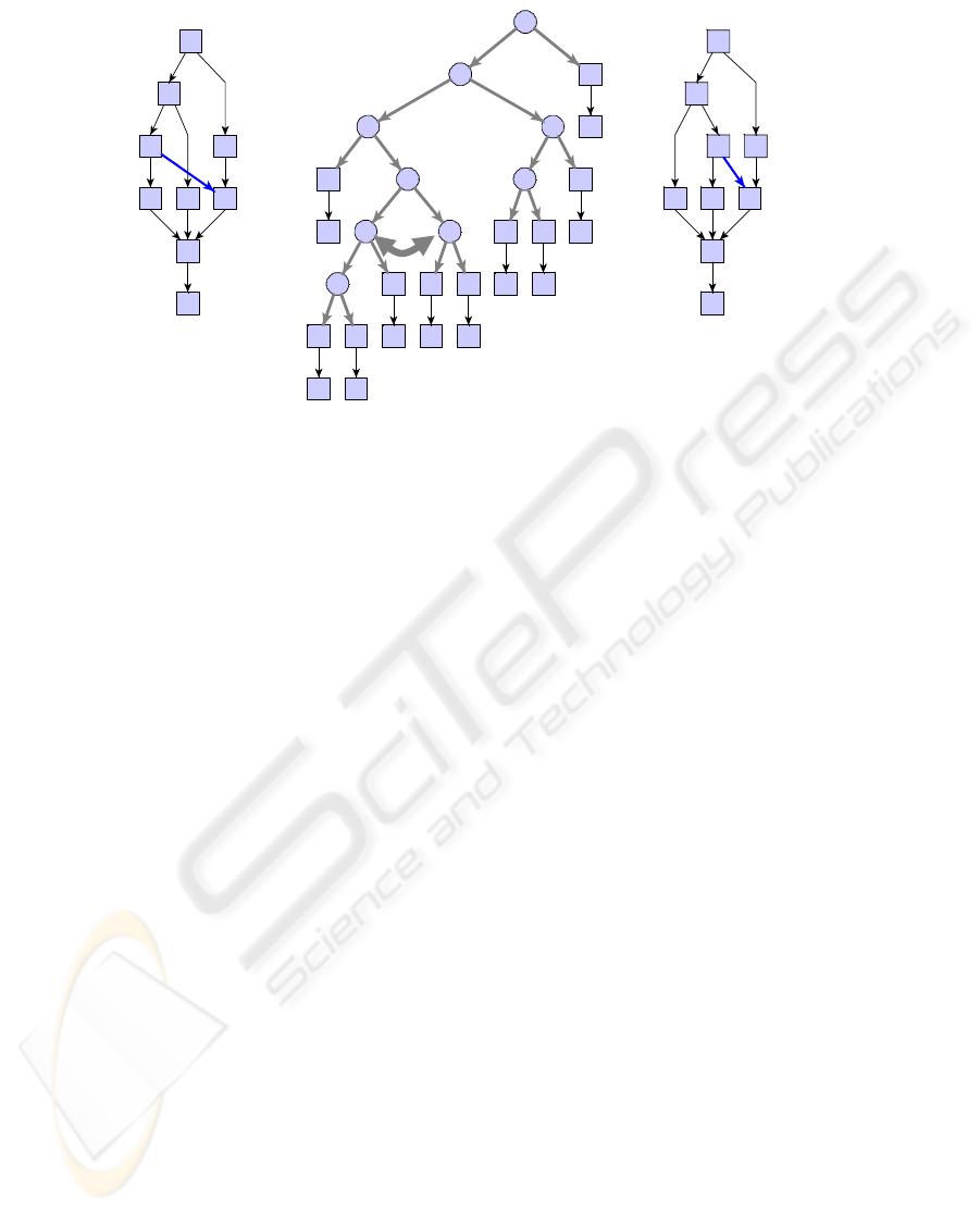
as depicted in Fig. 3.

The problem of maintaining the mental map when

conducting changes of the process logic has been rec-

ognized in the literature and different algorithms have

been presented in this context (e.g., Force-Scan or in-

cremental algorithms (Yang et al., 2004; Diguglielmo

et al., 2002)). However, all these approaches have

been applied to graphs with untyped nodes so far. For

this reason, it is also very interesting to analyze their

applicability on business processes.

2.3 Business Process Instances

Based on a process model, new process instances can

be created and executed during runtime. Since pro-

cess instances represent concrete executions of the

process model, the latter have to be enriched with

state information (e.g., node and edge markings) in

order to reﬂect the respective instances. The chal-

lenge is to display business process models together

with additional information (e.g., state markings or

instance-speciﬁc changes). An orthogonal aspect is

the way of visualizing process instances. They can be

displayed in a static way (displaying the instance and

its current state) or by using a dynamic layout (i.e., by

replaying the previous execution history of respective

instances along a time line).

2.4 Business Process Views

In practice process graphs are often very big and com-

plex (“wallpapers”). Thus users are overwhelmed

with information. Therefore a challenge for the vi-

sualization of business process graphs is to be able to

(dynamically) build up (dynamic) views on business

process graphs, i.e., to choose process objects along

certain criteria and to compose them in an appropri-

ate way. Criteria based on which process views can

be built may be (1)

object types

(we only display ob-

jects of a certain type, e.g., only nodes of type “activ-

ity” are displayed whereas nodes of types “data ele-

ment” or “actor” are hidden), (2)

static attribute val-

ues

(e.g., only manual activities are displayed whereas

automatic activities are hidden), and (3)

dynamic at-

tribute values

(e.g., displaying only those activities

which have not been worked on so far).

This technique is called

graph reduction

(Sadiq and

Orlowska, 2000). Another approach is

graph aggre-

gation

(Liu and Shen, 2003). Aggregation means to

nest certain objects (e.g., activities) to a complex ob-

ject (e.g., activity with underlying subprocess) and to

adapt activity attributes accordingly.

In order to provide a suitable framework for busi-

ness process layout it is extremely important to deeply

understand all these use cases and to provide appro-

priate approaches. In this paper we focus on the ﬁrst

use case (i.e., business process layout) to build up the

basis for the other use cases.

ICEIS 2006 - INFORMATION SYSTEMS ANALYSIS AND SPECIFICATION

206

Intended Change:

Graph after Relayout:

Insert new step

Figure 3: Overall Approach for Layouting Business Processes.

3 RELATED WORK

There are a lot of approaches dealing with graph lay-

out. In general, graph classes having certain prop-

erties are identiﬁed and layout algorithms based on

these properties are provided. These graph classes

and the respective algorithms comprise trees (Eades

et al., 1993), directed (acyclic) graphs (Sugiyama,

2002), planar graphs (de Fraysseix et al., 1988), and

series-parallel graphs (Hong et al., 1998). In the lit-

erature there are also approaches dealing with gen-

eral graphs, e.g., Heavy Duty Preprocessing, Spring

Embedder (Fruchterman and Reingold, 1991; Frick

et al., 1994), etc., There are also a few approaches

dealing with layouting process graphs (Six and Tol-

lis, 2002; Yang et al., 2004; Diguglielmo et al.,

2002). In (Six and Tollis, 2002) an approach is in-

troduced which determines a layout of the process

in linear time using existing partitioning information

(e.g., swimlanes). Yang et al (Yang et al., 2004) ad-

dress several problems described in connection with

the above use cases. In detail, they propose the so

called force scan algorithm which maintains the men-

tal map after changes. Furthermore the authors sug-

gest to use the ﬁsheye technique in order to overcome

the “wallpaper” problem. (Diguglielmo et al., 2002)

show how their tool jViews contributes to layout pro-

cess graphs. Using the incremental mode the mental

map of process graphs is maintained after changes. It

is also possible to impose a partitioning on the graphs

(e.g., swimlanes). An approach using a 3D represen-

tation of business processes including process analyis

results (e.g., throughput) is introduced in (Sch¨onhage

et al., 2000).

Though all of these approaches are very inspiring

they neglect the different semantics of the nodes and

edges within a business process. Therefore we will

make use of existing ideas and theoretical results but

combine and extend them towards an approach es-

pecially tailored for the layout of business process

graphs. Doing so might open a new interesting ap-

plication area for general graph drawing approaches.

4 BUSINESS PROCESS LAYOUT

In this section we present our approach for layout-

ing business process graphs which has been imple-

mented in the context the Proviado project on busi-

ness process visualization

. First of all, we intro-

duce a (canonical) process meta model describing the

different constructs which can be used for modeling

business processes. In order to provide a complete

formal basis for our further considerations we sim-

plify the meta model to some extend.

The partners are DaimlerChrysler, University of Ulm,

and University of Twente.

BUSINESS PROCESS VISUALIZATION - USE CASES, CHALLENGES, SOLUTIONS

207

Initiate change request Determine CR manager Instruct Expertise generate expertise (CAD)

generate expertise (car body)

generate expertise (motor)

CR initiator contact person CR manager

motor engineer

electronic engineer

car body engineer

change request

expertise (car body)

expertise (electronic)

expertise (motor)

Activity

Actor

Assignment

Data Element

Control flow

Edge

Synchronization

Edge

Data flow

Edge

StructureNode

Figure 4: Overall Approach for Layouting Business Processes.

4.1 Fundamentals

Within the canonical process meta model CP M we

specify A as the total set of all process activities, D

as the total set of process data elements, and W as

the total set of all actors involved in the execution of

any process model. Based on modeling elements of-

fered by CP M new

process models

can be deﬁned

(e.g., order procurement process in an enterprise or

treatment processes in a hospital).

Deﬁnition 1 (Process Model) A tuple PM = (A, D,

W, AT, CtrlE, CT, DataE, WorkE) is called a process

model with

• A ⊂Ais the set of activities, D ⊂Dis the set of data

elements, and W ⊂Wis the set of actors involved in the

execution of instances based on PM

• AT denotes the function which assigns to each activity

from A a particular type, i.e., AT: A →{Activity,

StructureNode, Start, End}; thereby struc-

ture nodes are used for structuring purposes (e.g., as split

or join nodes).

• CtrlE ⊂ A × A denotes the set of control edges in PM. A

control edge

a → b denotes that activity a must be completed before

activity b can start.

• CT denotes the function which maps control edges from

CtrlE onto their particular type, i.e., CT: CtrlE →

{Control, Sync, Loop}

• DataE ⊂ (A × D) ∪ (D × A) denotes the set of data

edges in PM; thereby D × A(A× D) describes a read

(write) access

• WorkE ⊂ W × A denotes the set of actor edges in PM; a

actor edge w → a denotes that activity a is worked on by

actor w.

An activity a ∈ A denotes a particular work

task within a process model PM, e.g., Instruct

Expertise (cf. Fig. 4). The direct successor of

this activity has activity type StructureNode (i.e.,

it is not associated with a speciﬁc work task). Since

this node has several outgoing control edges e

, ..., e

with CT(e

)=Control (i = 1, ..., n) it acts as a

split node of an alternate or parallel branching. Within

an alternate branching one branch is selected for ex-

ecution during runtime (e.g., based on process data)

whereas for parallel branchings all branches are exe-

cuted concurrently. Control edges describe the execu-

tion order between activities. They can be further dis-

tinguished into basic control edges, synchronization

edges, and loop edges. Synchronization edges deter-

mine the order of activities within different branches

of a parallel branching. Cyclic process structures can

be described by using loop backward edges. Besides

these control ﬂow constructs a process model con-

tains additional elements, e.g., data elements (e.g.,

change request in Fig. 4) and data edges. Read

(write) data edges describe which data elements are

read (written) by which activity. In Fig. 4, for ex-

ample, data element change request is written

by activity change request and read by activity

generate expertise (CAD). Finally, we de-

scribe which activity is worked on by which actors

by using actor assignments WorkE (e.g., actor car

body engineer works on activity Instruct

Expertise).

A process model can be (graphically) represented

as a process graph for which we want to ﬁnd a user-

friendly and process-adequate layout in the following.

The idea is to start with layouting a certain projec-

tion of the process consisting of

core

nodes and edges.

This layout is then stepwisely enhanced with the re-

maining

satellite

nodes and edges. In order to keep

the layout conﬁgurable we allow the user to specify

the sets of core and satellite objects.

Deﬁnition 2 (Core and Satellite Objects)

Let PM =

(A, D, W, AT, CtrlE, CT, DataE, WorkE) be a process model.

LetV:=(A∪ D ∪ W) and E := (CtrlE ∪ DataE ∪ WorkE).

Then PG = (V, E) denotes the process graph. Based on PG

the user can specify the set of core nodes CN by choosing

one of the sets A, D, and W. Then the set of core edges CE

and the set of satellite nodes (edges) SN (SE) can be derived

accordingly (i.e., CN = A =⇒ CE = CtrlE, CN = D =⇒ CE

= DataE, CN = W =⇒ CE = WorkE, SN:= V \ CN, SE:=

E \ CE).

ICEIS 2006 - INFORMATION SYSTEMS ANALYSIS AND SPECIFICATION

208

To achieve

structurally correct

process models the

associated process graph must obey certain correct-

ness constraints. We deﬁne

projections

on process

graphs which are used to introduce correctness con-

straints afterwards.

Deﬁnition 3 (Process Graph and Projections) Let

PM = (A, D, W, AT, CtrlE, CT, DataE, WorkE) be a process

model and let PG = (V, E) be the associated process graph

based on which we deﬁne different projections:

• PG

:= (V

) with V

= A and E

= {e

∈ CtrlE | CT(e) = Control} denotes the projection on

activities and control edges of type Control.

• PG

Sync

:= (V

Sync

) with E

Sync

:= E

∪{e ∈

CtrlE | CT(e) = Sync} denotes the projection on PG

plus sync edges.

• PG

Loop

:= (V

Loop

) with E

Loop

:= E

Sync

∪{e

∈ CtrlE | CT(e) = Loop} denotes the projection on

Sync

plus loop edges. We denote PG

Loop

as control

ﬂow skeleton.

A process graph must adhere the following con-

straints in order to represent a structurallycorrect pro-

cess model (e.g., avoiding deadlock causing cycles).

Deﬁnition 4 (Correctness of a Process Graph)

Let

PG = (V, E) be a process graph and PG

:= (V

Sync

:= (V

Sync

), PG

Loop

:= (V

Loop

)be

the projections as deﬁned in Def. 3. Then PG is a correct

process graph iff the following constraints hold:

1. Unique Start and End Node:

∃ s ∈ V

:  ∃ e = (v’, s) with CT(e) ∈{Control,

Sync}∈E, v’ ∈ V

∧

∃ e ∈ V

:  ∃ e = (e, v”) ∈ E with CT(e) ∈

{Control,Sync},v”∈ V

∧ s = e

2. Connectivity:

is connected ∧

∀s ∈ V \ V

: (∃e =(s, v) ∈ E ∨∃e =(v, s) ∈

E), v ∈ V

3. Synchronization: Control edges between activities from

different parallel branches are only of type Sync, for-

mally:

∀e =(a

) ∈ E with a

∈ V

∧ a

∈

(succ*(PG, a

) ∪ pred*(PG, a

)): CT(e) = Sync

where

• succ*(PG, n):= succ(PG, n) ∨ succ(PG, succ*(PG, n))

with

succ(PG, n):={n’ ∈ V

|∃e = (n, n’) ∈ E with CT(e)

∈{Control, Sync}}

• pred*(PG, n):= pred(PG, n) ∨ pred(PG, pred*(PG, n))

with

with pred(PG, n):={n’ ∈ V

|∃e = (n’, n) ∈ E with

CT(e) ∈{Control, Sync}}

4. Deadlockfree: PG

Sync

is an acyclic graph, i.e., the

use of control and sync edges must not lead to deadlock-

causing cycles.

After introducing the necessary fundamentals we

nowdescribe our approachfor layoutingbusiness pro-

cess graphs. Generally, users can conﬁgure which

nodes and edges are considered as core and which are

considered as satellite objects. This inﬂuences the re-

sulting process graph layout. As we know from our

practical studies in most cases users prioritize an ad-

equate layout of the control ﬂow skeleton (i.e., the

work tasks themselves and the order in which they

are to be carried out). For this we select the activi-

ties as the set of core nodes (i.e., CN = A). Thus

the set of core edges contains the control edges (i.e.,

CE = CtrlE). Accordingly, the set of satellite nodes

comprises data and actor nodes (i.e., SN = D ∪ W )

and the set of satellite edges contains data and actor

edges (i.e., SE = DataE ∪ WorkE). Due to lack of

space in this paper we present our approach for focus-

ing on the control ﬂow ﬁrst and enhancing it with data

and actor elements in the following. Nevertheless,

this approach can be transferred to other methodolo-

gies (e.g., starting with the data ﬂow graph) as well.

4.2 On Layouting Process Graphs

As discussed above often an appropriate layout of the

control ﬂow skeleton is fundamental for the process

graph layout. Therefore we start with layouting the

control ﬂow skeleton followed by the placement of

satellite objects. Let PG =(V,E) be a process graph

and CN , CE, SN , SE be the set of core and satel-

lite nodes (edges) as speciﬁed by the user (in the fol-

lowing: CN = A, CE = CtrlE, SN = D ∪ A,

SE = DataE ∪ WorkE). We start with ﬁnding an

adequate layout of the control ﬂow skeleton PG

Loop

Adequate means (at least) to focus on the control ﬂow

and to minimize edge crossings (Purchase, 2002). Be-

sides these two most important aspects other esthetic

criteria exist (e.g., mimizing the layout size). Due to

lack of space we omit further details here.

First of all, comparable to heavy duty preprocess-

ing approaches, we determine PG

(cf. Def. 3).

We can show that PG

(together with correctness

constraints 1 – 4) constitutes a series-parallel graph,

i.e., it can be constructed by serial and parallel con-

struction. This construction is reﬂected by the

struc-

ture tree

(Hong et al., 1998). For example, Fig. 5

shows the structure tree for an abstract process. Since

is series-parallel (and therefore planar) it can

be drawn without any edge crossings (e.g., using

the Sugiyama algorithm with Barycenter crossing re-

duction and coordinate assignment using (Sugiyama,

2002; Brandes and K¨opf, 2002)).

However, if we also consider synchronization

edges (graph projection PG

Sync

) edge crossings may

occur (cf. Fig. 5), i.e., crossings between sync edges

or crossings between sync and control edges of type

Control. As it can be seen from Fig. 5 the number

of (sync) edge crossings depends on the aligment of

the associated parallel branches. Therefore our aim

is to ﬁnd an alignment of the parallel branches for

which the number of (sync) edge crossings becomes

BUSINESS PROCESS VISUALIZATION - USE CASES, CHALLENGES, SOLUTIONS

209

Abstract Process PG

Sync

: Structure Tree:

S S

Abstract Process PG’

Sync

(After Permutation):

permutation

Figure 5: PG

with Associated Structure Tree.

minimal. In the following we use the correlation be-

tween the order of branches in the structure tree and

the alignment of the parallel branches in PG

.By

permuting the order of the branches in the structure

tree we obtain the different possible alignments of the

parallel branches in PG

. Since we must not change

the original order of working tasks we only allow to

permute the order ot the siblings of parallel composi-

tion nodes (cf. Fig. 5).

Among all permutations the layout with minimal

number of edge crossings can be found. In gen-

eral, routing of loop edges can be handled analo-

gously. However, the evaluation of the resulting lay-

out with respect to the number of edge crossings be-

comes more complex since we are confronted with

different types of edge crossings. Therefore we need

a more sophisticated evaluation metrics minimizing

the number cross

sync

of sync edge crossings plus

the number cross

loop

of loop edge crossings where

users can weight the numbers with priorization fac-

tors d

for sync edges and d

for loop edges (i.e.,

min(d

∗ cross

sync

+ d

∗ cross

loop

)).

4.3 Satellite Objects

After determining the layout for PG

Loop

the control

ﬂow skeleton is enhancedwith information about data

ﬂow and actor assignments. This remaining informa-

tion is captured by the sets of satellite nodes and edges

(i.e., SN = D ∪ W and SE = DataE ∪ WorkE). There

are different possibilities for integrating the satellite

objects into the existing control ﬂow skeleton layout.

We sketch them and describe which factors may in-

ﬂuence the decision for one of these possibilities as

well as their advantages and drawbacks. Basically,

we distinguish between a

local alignment

and a

global

alignment

of satellite objects. Local alignment means

that the satellite objects belonging to a work task are

aligned in the “surrounding” of the work task what

may lead to duplication of satellite objects. Choosing

global alignment each object is unique und connected

to one ore more activities by the respective edges.

Local Alignment: If we choose local alignment the

satellite objects associated with a certain activity are

aligned “around” this activity. Then the activity to-

gether with its satellite objects can be seen as one

(complex) activity. Inserting this complex activity

into the control ﬂow skeleton can be achieved by

shifting the other activities in order to obtain the nec-

essary space. This can be done, e.g., with the Force-

Scan algorithm for maintaining the mental map after

changes (Yang et al., 2004). The advantage of local

alignment is that the number of edge crossings is not

increased by the alignment of the satellite objects. A

possible drawback is that users may loose the process

overview or the correlation between the different du-

plicates of satellite objects is not visible.

Global Alignment: The ﬁrst possibility is that users

manually

align satellite objects, i.e., they take the con-

trol ﬂow skeleton layout and place the satellite objects

together with the respective edges manually around

the skeleton, Then satellite objects, e.g., data ele-

ments, are placed “around” the skeleton. Reasons for

this approach may be that there are only few satellite

objects or the user prefers a special alignment. An-

other approach is to treat the alignment of satellite

objects as dynamic changes and to apply one of the

algorithms proposed in the literature, e.g., the Force-

ICEIS 2006 - INFORMATION SYSTEMS ANALYSIS AND SPECIFICATION

210

Scan algorithm (Yang et al., 2004).

One disadvantage of all global approaches is that

the number of edge crossings is potentially increased.

To overcome this limitation the insertion of the satel-

lite edges (i.e., data ﬂow or work assignment edges)

could be already integrated in the permutation step in-

troduced in Section 4.2.

5 SUMMARY AND OUTLOOK

We have discussed several use cases related to

the visualization and layout of business process

graphs which have been identiﬁed within the Provi-

ado project (process visualisation in the automotive

domain) in cooperation with DaimlerChrysler Re-

search Ulm. Furthermore, a layout approach which

exploits the different semantics of the nodes and

edges of a process graph has been introduced.

This approach can be improved by using already

existing information (e.g., knowledge about process

meta model properties or existing layout information)

within the algorithm. In our approach the following

meta model properties could be useful for a respec-

tive improvement: We start with layouting the series-

parallel control ﬂow skeleton of a business process.

For certain process meta models like BPEL4WS or

WSM Nets (Rinderle et al., 2004) it can be shown

that they are

block-structured

, i.e., they are not only

series-parallel but possess a nested structure (i.e., for

each split node a unique join node can be found and

vice versa). If we know that the business process

was modeled in a block-structured way we can use

this information in constructing the series-parallel (or

block-structured) control ﬂow skeleton. If we know

that the process was modeled according to an acyclic

process meta model, e.g., Activity Nets as used in

IBM Websphere products, we can use this informa-

tion to abstain from the last step of inserting the loop

edges into the directed ayclic control ﬂow skeleton.

The current implementation of our approach com-

prises a visualization component for process graphs

based on the scalable vector graphic (svg) format.

Furthermore we plan to integrate this component

within our adaptive process management system

ADEPT2. Based on this we can, for example, eval-

uate approaches for maintaining the mental map after

process changes (Rinderle et al., 2004).

REFERENCES

Bobrik, R., Reichert, M., and Bauer, T. (2005). Require-

ments for the visualization of system-spanning busi-

ness processes. In DEXA’05, pages 948–954.

Brandes, U. and K¨opf, B. (2002). Fast and simple horizontal

coordinate assignment. In GD01.

de Fraysseix, H., Pach, J., and Pollack, R. (1988). Small

sets supporting fary embeddings of planar graphs. In

STOC’88, pages 426–433.

Diguglielmo, G., Durocher, E., Kaplan, P., Sander, G., and

Vasiliu, A. (2002). Graph layout for workﬂow appli-

cations with ILOG jViews. In Proc. GD02.

Eades, P., Lin, T., and Lin, X. (1993). Two tree drawing

conventions. Computional Geometry & Applications,

3(2):133–153.

Fleischer, R. and Hirsch, C. (2001). Graph drawing and

its applications. In Grawing Graphs: Methods and

Models, pages 1–21.

Frick, A., Ludwig, A.,and Mehldau, H. (1994). A fast adap-

tive layout algorithm for undirected graphs. In GD94.

Fruchterman, T. and Reingold, E. (1991). Graph drawing

by force-directed placement. Software Practice and

Experience, 21(11):1129–1164.

Hong, S., Eades, P., Quigley, A., and Lee, S. (1998). Draw-

ing algorithms for series-parallel digraphs in two and

three dimensions. In Proc. GD98, pages 198–209.

Kikusts, P. and Rucevskis, P. (1995). Layout algorithms

of graph-like diagrams for GRADE windows graphic

editors. In Proc. GD95, pages 361–364.

Liu, D. and Shen, M. (2003). Workﬂow modeling for vir-

tual processes: An order–preserving process–view ap-

proach. Information Systems, 28(6):505–532.

Purchase, H. (2002). Metrics for graph drawing aesthetics.

Visual Languages and Computing, 13:501–516.

Reichert, M. and Dadam, P. (1998). ADEPT

flex

- sup-

porting dynamic changes of workﬂows without losing

control. JIIS, 10(2):93–129.

Rinderle, S., Reichert, M., and Dadam, P. (2004). Flexi-

ble support of team processes by adaptive workﬂow

systems. DPD, 16(1):91–116.

Sadiq, W. and Orlowska, M. (2000). Analyzing process

models using graph reduction techniques. Information

Systems, 25(2):117–134.

Sch¨onhage, B., van Ballegooij, A., and Elliens, A. (2000).

3D gadgets for business process visualization - a case

study. In Web3D – VRML 2000, pages 131–138.

Six, J. and Tollis, I. (2002). Automated visualization of

process diagrams. In Proc. GD01, pages 45–59.

Sugiyama, K. (2002). Graph Drawing and Applications

for Software and Knowledge Engineering. Series on

Software Eng. & Knowledge Eng. World Scientiﬁc.

Wittenburg, K. and Weitzman, L. (1996a). Process visual-

ization in ShowBiz. In Proc. GD96.

Wittenburg, K. and Weitzman, L. (1996b). Relational gram-

mars: Theory and practice in a visual language inter-

face for process modeling. In In Proc. Workshop on

Theory of Visual Languages, Gubbio, Italy.

Yang, Y., Lai, W., Shen, J., Huang, X., J.Yan, and Setiawa,

L. (2004). Effective visualisation of workﬂow enact-

ment. In APWeb’04, pages 794–803.

BUSINESS PROCESS VISUALIZATION - USE CASES, CHALLENGES, SOLUTIONS

211