SEGMENTATION ALGORITHMS FOR EXTRACTION OF

IDENTIFIER CODES IN CONTAINERS

Juan A. Rosell Ortega, Alberto J. P

erez Jim

enez and Gabriela Andreu Garc

ıa

Grupo de Visi

on por Computador , DISCA.

Universidad Polit

ecnica de Valencia

Camino de Vera s/n, Valencia, Spain

Keywords:

segmentation algorithms, characters.

Abstract:

In this paper we present a study of four segmentation algorithms with the aim of extracting characters from

containers. We compare their performance using images acquired under real conditions and using results of

human operators as a model to check their capabilities. We modiﬁed the algorithms to adapt them to our needs.

Our aim is obtaining a segmentation of the image which contains all, or as much as possible, characters of

the container’s code; no matter how many other non relevant objects may appear; as irrelevant objects may be

ﬁltered out by applying other techniques afterwards. This work is part of a higher order project whose aim is

the automation of the entrance gate of a port.

1 INTRODUCTION

A lot of work has been done in the area of com-

paring segmentation algorithms attending to different

categorizations. There have been a number of sur-

vey papers on thresholding; for instance, in (Sezgin

and Sankur, 2004), a taxonomy of thresholding tech-

niques is presented, and several algorithms are cate-

gorized, expressed under a uniform notation and com-

pared according to uniﬁed criteria.

We present in this paper, however, a comparison of

four segmentation algorithms aimed to deal with pic-

tures containing container code characters. The goal

of the work is not to compare the performance of the

algorithms in general conditions, but with a wide set

of images that correspond to images representative of

what the system will have to deal with in real situa-

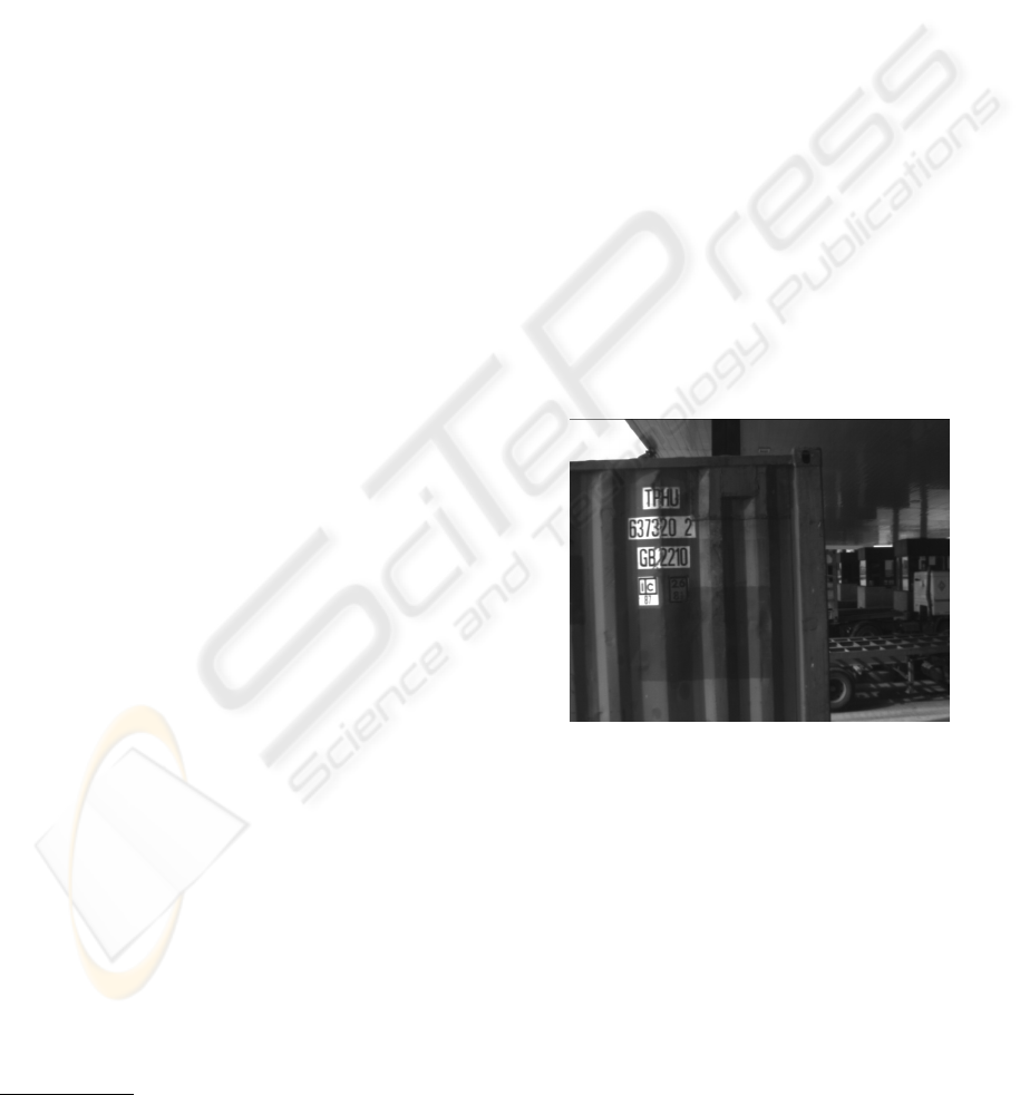
tions (see ﬁgure 1 as a sample of the images we used).

Our criterion to check results was comparing the re-

sults of each algorithm with the results obtained by a

human operator.

Currently in most trading ports, gates are con-

trolled by human inspection and manual registration.

This process can be automated by means of com-

puter vision and pattern recognition techniques. Such

a prototype should be built by developing different

This work has been partially supported by grant

FEDER-CICYT DPI2003-09173-C02-01.

Figure 1: Sample image of a container.

techniques, such as image preprocessing, image seg-

mentation, feature extraction and pattern classiﬁca-

tion. The process is complex; because it has to deal

with outdoor scenes, days with different climatology

(sunny, cloudy...), changes in light conditions (day,

night) and dirty or damaged containers.

A ﬁrst approach to the process of code detection is

presented in a previous work (Salvador et al., 2001)

and the overall process is discussed also in (Salvador

et al., 2002). In these works, authors use a morpho-

logical operator called top-hat to segment the same

kind of images as we do. This operator has to be

applied twice per image, once trying to distinguish

375

A. Rosell Ortega J., J. Pérez Jiménez A. and Andreu Gar

cıa G. (2006).

SEGMENTATION ALGORITHMS FOR EXTRACTION OF IDENTIFIER CODES IN CONTAINERS.

In Proceedings of the First International Conference on Computer Vision Theory and Applications, pages 375-380

DOI: 10.5220/0001365303750380

 SciTePress

clear objects on a dark background and again looking

for dark objects on a clear background. Though this

method had good results, we tried to improve their

performance by using the methods we expose in this

article.

Another work (Atienza et al., 2005), presents an

investigation which is currently being developed. The

aim of the authors of this paper is to use the optical

ﬂow in order to shrink the area where the container

code could be found and speed up the segmentation

process; however, the method is time consuming and

an effort is currently being done in order to optimize

it.

Our aim was ﬁnding a suitable successful segmen-

tation algorithm for the process of code detection

mentioned previously. To achieve this goal, we tested

several segmentation algorithms found in the litera-

ture. By comparing the results obtained from the four

algorithms we tested, we extracted conclusions about

which could perform better under the conditions we

work with. We wanted to know which algorithm (or

algorithms) could ﬁt better to our needs, and, if it was

the case, which we could merge into one, that could

produce better results than any other algorithm on its

own.

In summarize, we are looking for an algorithm that

meets the following constraints:

• It must detect all characters in the code, or as much

as possible.

• It must ﬁnd characters independently of their

colour (white characters on a dark background and

vice versa).

• It must be independent of image light conditions.

• It must create the minimal list of found objects; as

segmentation algorithms will always ﬁnd objects

which are not relevant (see picture 4), the best will

be the one which creates a list that only contains

objects which correspond to characters in the code.

We have organized the paper as follows, in next

section we describe the algorithms used, section 3 will

describe the pictures used and the experiments done;

in section 4 we show the results we obtained in the

experiments and in section 5 we discuss our conclu-

sions.

2 ALGORITHMS

As mentioned before, we have implemented and com-

pared four different algorithms. In this section we

describe them brieﬂy and we give a formal introduc-

tion to each one. These algorithms are: the water-

shed algorithm (Beucher and C-Lantu

ejoul, 1979),

LAT (Kirby and Rosenfeld, 1979), local variation al-

gorithm (Felzenszwalb and Huttenlocher, 1998) and

thresholding algorithm. Each algorithm represents a

different approach to the segmentation problem. Our

election was based on previous knowledge of the al-

gorithms and also on the comparison of the literature

describing them.

2.1 Watershed

Application of the watershed transform to image

segmentation was proposed in (Beucher and C-

Lantu

ejoul, 1979). The algorithm takes a gray scale

image and considers it as a topographic surface. A

process of ﬂooding is simulated on this surface; dur-

ing this process two or more ﬂoods coming from dif-

ferent basins may merge. To avoid this, dams are built

on the points where the waters ﬂooding from different

basins meet; at the end of the algorithm, only dams

are over water level. These dams deﬁne the watershed

of the image.

One of the problems of this algorithm is over seg-

mentation. We took no direct action to avoid it; in-

stead, we used ﬁlters (as mentioned later in section 3)

to remove regions from the segmentation which were

not relevant.

2.2 LAT

This algorithm was proposed by Kirby and Rosenfeld

in (Kirby and Rosenfeld, 1979). Adaptive threshold-

ing typically takes a grayscale or colour image as in-

put and, outputs a binary image representing the seg-

mentation. For each pixel in the image, a threshold

has to be calculated. If the pixel value is below the

threshold it is set to the background value, otherwise

it assumes the foreground value; or vice versa.

The algorithm uses a window w

n×n

) of n×n el-

ements (the neighbourhood to consider for each pixel

), n is odd in order to centre the matrix on the con-

sidered pixel of the image. This matrix is used to cal-

culate statistics to examine the intensity f(p

) of the

local neighbourhood of each pixel p

. The statistic

which is most appropriate depends largely on the in-

put image. We used the mean of the local intensity,

computed as:

µ(p

n ∗ n

∗



∈w

n∗n

)

f(p

) (1)

The size of the considered neighbourhood has to

be large enough to cover sufﬁcient foreground and

background pixels, otherwise a poor threshold is cho-

sen. On the other hand, choosing regions which are

too large can violate the assumption of approximately

uniform illumination.

A factor k may be used to adjust the comparison of

the statistic used with the pixel intensity value. This

VISAPP 2006 - IMAGE ANALYSIS

376

factor multiplies the average gray level when compar-

ing it to the gray level of the pixel.

The algorithm forms the segmentation of image I

by calculating the union of the segmentations result of

using different factors, converting image I into bina-

rized image I



. Each pixel in I



is deﬁned depending

on its counterpart in I:

∀p



∈ I



= thr(p

):p

∈ I (2)

with thr(p

) deﬁned as:

thr(p



1,ifµ(p

) ≥ k × f (p

)

0, otherwise

(3)

We looked for connected regions after each thresh-

olding and merged the results of each segmentation

with the previous. So, if a set of pixels belonged to

any region for a certain segmentation, they did in the

ﬁnal segmentation.

2.3 Thresholding

It is the simplest approach to image segmentation.

The input is a gray level image I and the output is a

binary image I



representing the segmentation where

black pixels correspond to background and white pix-

els correspond to foreground (or vice versa). In a sin-

gle pass, each pixel in the image is compared with a

given threshold k which is a gray level. If the pixel’s

intensity f (p

) is higher or equal to the threshold k,

the pixel p

is set to, say, white in the output. If it is

under k, it is set to black. The segmentations result of

applying each threshold k are joined in a similar way

as in LAT.

2.4 Local Variation

The algorithm we implemented is based on the work

introduced in (Felzenszwalb and Huttenlocher, 1998).

An important feature of this algorithm over the other

three is that it does not need a priori information on

which the colour of the objects is.

Felzenszwalb’s approach consists on considering a

criterion for segmenting images based on intensity

differences between neighbouring pixels. The algo-

rithm is based on the idea of partitioning an image

into regions, such that for each pair of regions the

variation between them is bigger than the variation

within regions. The criterion for determining the sim-

ilarity of image regions is based on measures of im-

age variation. The measure of the internal variation of

a region is an statistic of the intensity differences be-

tween neighbouring pixels in the region. The measure

of the external variation between regions is the mini-

mum intensity difference between neighbouring pix-

els along the border of the two regions. The original

algorithm uses two parameters, the minimum size of

the regions in the ﬁnal result, and one used to smooth

the image before processing it.

Felzenszwalb starts by creating a graph that rep-

resents the image. Arches in the graph are given a

weight that corresponds to the difference in inten-

sity of pixels represented by their vertices. Arches

join pixels to their 8-connected neighbourhood. To

achieve the fastest ordering, original authors recom-

mend in their paper the bucket sort algorithm (Cor-

men et al., 1990). After this step, all arches are or-

dered by non-decreasing weight. The algorithm then

follows by taking an arch at a time and compare the

regions to which each of its ends belongs to. Both

regions will be merged if they accomplish with the

established criteria. The output of the algorithm is a

set of regions in which the image is segmented.

Formally, the graph G on the image I is deﬁned as

follows. Each pixel p

in the image will correspond to

a vertex v

in the graph. Arches connect neighbouring

pixels and each arch is assigned with a weight. The

function used to calculate the weight of the arches is

deﬁned as follows:

w(v



|I(v

) − I(v

)|,if(v

) ∈ E

∞, otherwise

(4)

E is the set of all edges deﬁned. As we said, for

each vertex v

in the graph exists a pixel p

in the im-

age, thus, E is the set of all arches connecting ver-

tices in G for some given distance d (in our case,

d =1, so we only consider immediate neighbours),

E = {(v

):||p

− p

|| ≤ d}. The segmentation

S of an image I is then a partition of I with a corre-

sponding set of edges, G ⊆ E, such that each compo-

nent C in the segmentation, C ∈ S, corresponds to a

connected component in the graph G.

We used the mean intensity of the region to decide

whether two regions should merge or not instead of

the variance as in the original algorithm. Following

a similar approach as Felzenszwalb does in his algo-

rithm, we decided that two different regions should

join into one if the mean intensity of both regions is

similar. Another difference is that we didn’t use a

minimum size of region, in fact, regions were merged

until the process reaches a situation in which no more

regions could be merged.

We modiﬁed the original algorithm because it was

difﬁcult to ﬁnd values for its parameters that could

perform well with the variety of images we had. We

used the mean of gray intensity of the region which,

after several tests, proved to perform similar to the

original algorithm. In our case, however, we used one

parameter, the percentage of similarity k. For each

value of k we have a different segmentation, all these

resulting segmentations are then joined as in the pre-

vious algorithms.

SEGMENTATION ALGORITHMS FOR EXTRACTION OF IDENTIFIER CODES IN CONTAINERS

377

3 EXPERIMENTS

We used 309 real images with each algorithm in order

to obtain experimental results to evaluate their perfor-

mance. These images represent truck containers and

have a size of 720 × 574 pixels in gray levels. They

were acquired under real conditions in the admission

gate of the port of Valencia. In ﬁgure 2, there is a

sample of the kind of pictures we used. They were

selected randomly between a large set of pictures, but

we assured all variability was represented in this set

of pictures (sunny or cloudy days, daytime or night-

time, damaged containers...).

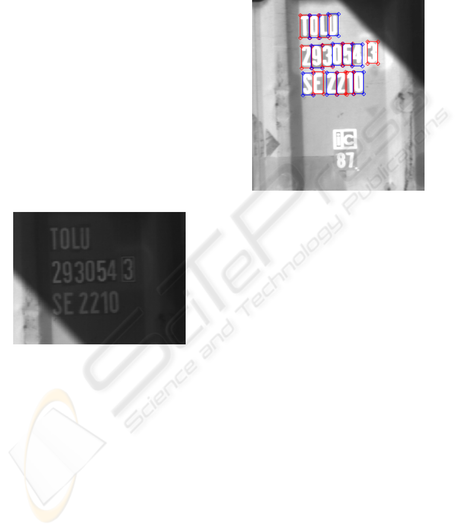
In order to extract conclusions about the perfor-

mance of the algorithms; we labelled by hand all char-

acters in the images. We made this by drawing the in-

clusion box of each character in the image and saving

the coordinates, an example is shown in ﬁgure 3. As

a result of this labelling, we had the number of code

characters and the coordinates of the inclusion boxes

of each code character of each image. We automated

the processing of the experiment’s results.

Figure 2: A sample container, image zoomed in to show

only the area of the container’s code.

During experiments, algorithms were not provided

with concrete information about light conditions of

each image during their executions, because we

wanted to know how they would perform in real con-

ditions.

Algorithms’ parameters vary in a range wide

enough to cover all possible situations. As watershed

needs no arguments, we need not to use any parame-

ter. For LAT we used a value of k in the range of

[0.9, 1.6] with a step value of 0.03, which makes a to-

tal of 23 segmentations per image. For thresholding

algorithm we used a value of k ranging from 20 to 220

with a step value of 5, which makes up 40 segmenta-

tions per image. With Local Variation we used a value

of the similarity percentage in the range [70%, 85%]

with a step of 5% which makes a total of 4 segmen-

tations. Besides, each algorithm (but Local Variation)

had to be executed twice per image, once searching

for white characters and again for black characters.

Because of its nature, Local Variation ﬁnds directly

characters no matter which colour they are.

Figure 3: Inclusion boxes drawn by a human operator.

We obtained of each algorithm a list of found ob-

jects in each image. These objects correspond to con-

nected regions with equal gray intensity levels. Some

of these objects were not relevant to our purposes, and

some others corresponded to the code characters.

As it may be seen in picture 4, the number of ob-

jects is bigger than the number of code characters.

We evaluate the good or bad performing of algo-

rithms depending on the amount of code characters

included in the list of objects it found, not in the total

amount of found objects. Other procedures applied

after this segmentation step may be implemented to

reduce the number of irrelevant objects. With a geo-

metrical ﬁlter we removed any object which did not

meet the geometrical properties we expect of any

character in the code (aspect ratio, minimum area

size, height and width).

Other ﬁlters could have also been applied. For in-

stance, contrast ﬁlters or classiﬁer ﬁlters, that would

remove all objects which were not classiﬁed as a char-

acter. But there was the chance that ﬁlters hided errors

of the algorithms or add their own errors to the ﬁnal

result, masking the performance of the algorithms.

We set up a method to compare the inclusion boxes

calculated by each algorithm with the inclusion boxes

we had labelled manually. We considered the algo-

rithm had done a hit if the inclusion box it had calcu-

lated and the hand labelled inclusion box overlapped

one on each other in a certain percentage.

We obtained the number of hits per image of each

algorithm, the number of failures (labels which had

no counterpart in the result list of the algorithm), the

VISAPP 2006 - IMAGE ANALYSIS

378

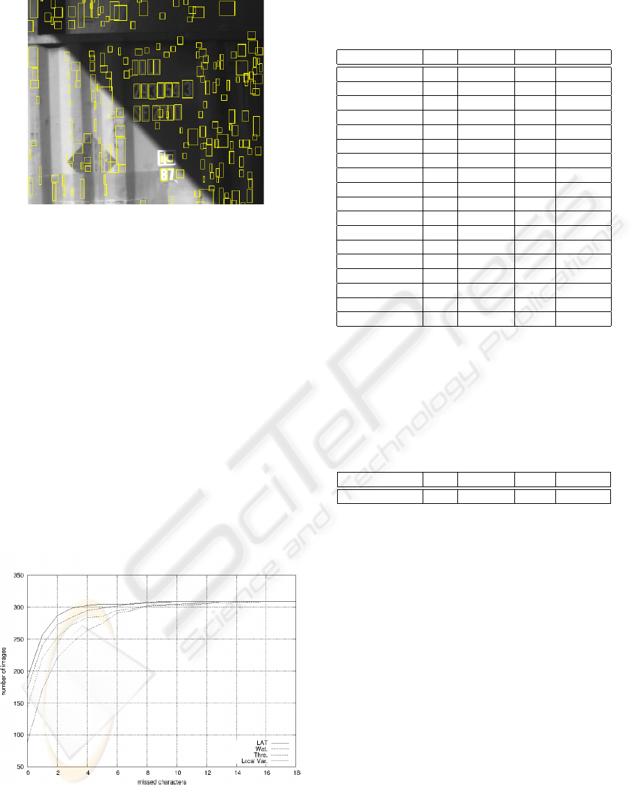
Figure 4: Inclusion boxes drawn by LAT.

total amount of objects found by the algorithm and

the total time spent.

4 RESULTS

The ﬁrst results we obtained are shown in table 1. In

this table, we see that LAT is the one that performs

better. It is the one that gets the biggest amount of

images with up to 4 characters missed. Watershed is

the second algorithm that performs best. On the other

hand, the adaptation we made of the algorithm of lo-

cal variation has an erratic behaviour, this is maybe

due to the fact that we were only using the mean aver-

age of the regions to decide whether to merge them or

not (recall section 2.4). Values on table 1 are plotted

in ﬁgure 5.

Figure 5: Cumulative plot of images according to the num-

ber of missed characters.

In table 2, we show the mean time of execution for

each algorithm (in seconds). LAT is the fastest, and

Table 1: Performance of the algorithms. Amount of images

according to the number of missed characters.

Missed characters LAT Watershed Thres. Local var.

0 189 173 143 88

1 68 68 78 84

2 30 32 32 49

3 12 12 20 24

4 4 10 11 19

5 2 4 2 11

6 0 3 9 16

7 0 4 3 4

8 2 2 4 8

9 1 1 1 1

10 1 0 1 1

11 0 0 0 1

12 0 0 2 2

13 0 0 1 1

14 0 0 1 0

15 0 0 0 0

16 0 0 1 0

17 0 0 0 0

its execution time is far away from the amount of time

needed by the local variation algorithm(the slowest)

to execute, which is also the algorithm with the worst

performance.

Table 2: Mean time of execution of the algorithms.

Mean time \ Alg. LAT Watershed Thres. Local var.

seconds 1.31 7.11 1.78 26.54

After these ﬁrst results, we thought it would be a

good idea trying to merge the best two algorithms

into one, in order to get beneﬁts from both. Merg-

ing the algorithms consisted on applying them both

on the same image and take results together applying

the ﬁlters to the this merged output.

We repeated the tests taking both LAT and wa-

tershed algorithm as the basis of our merged algo-

rithm. We merged also LAT and thresholding algo-

rithm, though the last is not the second best, it is

fast and this could mean more hits with less execu-

tion time. We thought this was a good enough reason

as to give it a try. We made also a test joining these

three algorithms into one.

We were puzzled at ﬁrst by the poor performance

of the local variation algorithm. We concluded we

needed to adapt the same philosophy we used for LAT

and let the algorithm iterate several times over the

same image looking for objects, and using in each it-

eration a different criterion (k) to merge regions. In

table 3 we compare the results we obtained with the

LAT-Watershed algorithm, the modiﬁed local varia-

tion algorithm and the LAT-Watershed-Thresholding

SEGMENTATION ALGORITHMS FOR EXTRACTION OF IDENTIFIER CODES IN CONTAINERS

379

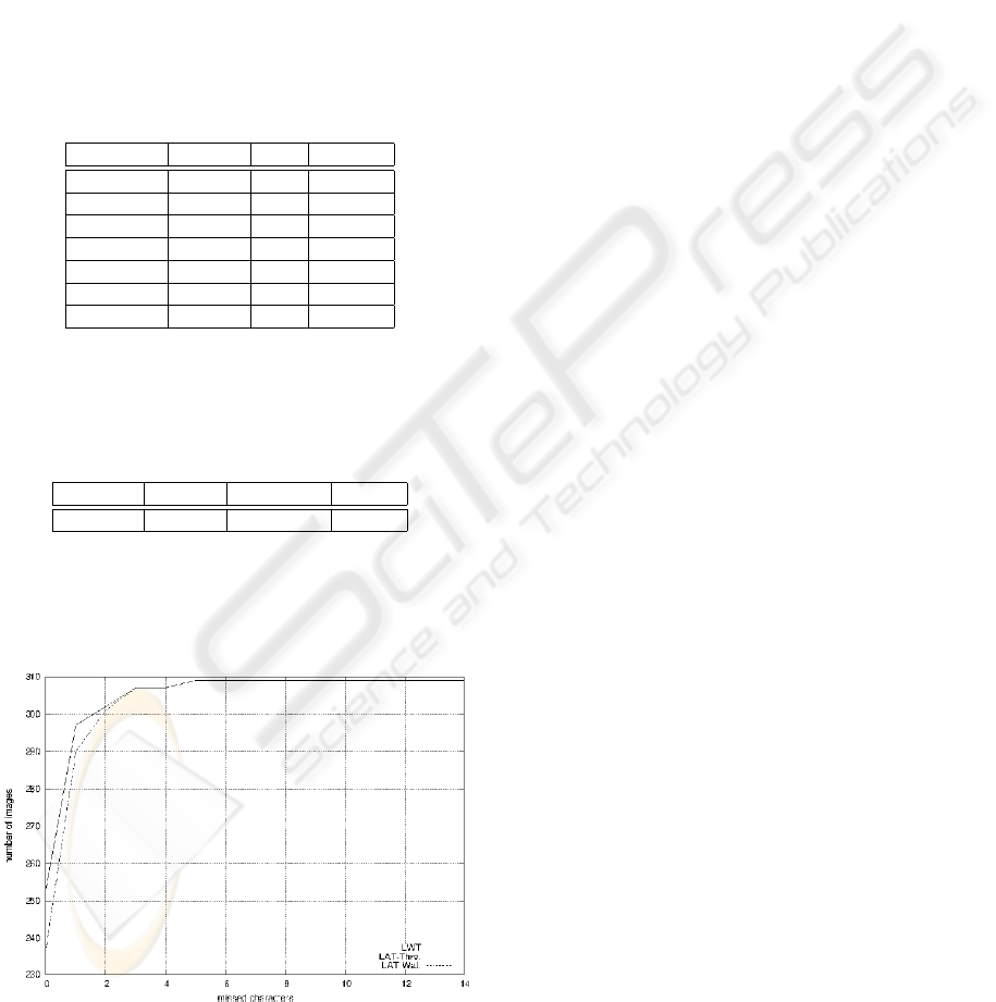
algorithm (called LWT in the table). We can see also

that the algorithm made by joining watershed algo-

rithm and LAT performs better than the rest, and with

the same performance as the serialization of thresh-

olding algorithm with watershed algorithm and LAT.

In table 4 we show the times consumed by the

merged versions; the algorithm formed by the seri-

alization of LAT and thresholding algorithm is a bit

quicker than the sum of the times of both algorithms

taken separately. In 6 we can see a graphical compar-

ison of the improved algorithms.

Table 3: Performance of the improved algorithms, com-

pared with the two algorithms with best results.

Missed char. LAT-Thr. LWT LAT-Wat.

0 237 253 253

1 53 44 44

2 11 5 5

3 6 5 5

4 0 0 0

5 2 2 2

6 0 0 0

Table 4: Mean time of execution of the improved algo-

rithms.

Mean time LAT-Thr. Lat-Wat-Thr. Lat-Wat

seconds 2.67 10.18 8.19

Figure 6: Cumulative plot of images according to the num-

ber of missed characters, for the improved algorithms.

5 CONCLUSIONS

We present a comparison of four segmentation algo-

rithms. We checked their performance dealing with

pictures with character codes on containers. We used

309 real images selected randomly between a large

set of real images, and compared the performance of

algorithms against the results given by a human oper-

ator.

Our effort was driven by the fact that we wanted to

ﬁnd the algorithm that did not miss any character (or

the lowest amount possible) in the container’s code.

Our evaluation of the algorithms, then, penalties al-

gorithms which lose characters in the code. Future

efforts will focus on developing ﬁlters which allow

us to remove regions which are not relevant to our

search.

As results show, LAT or watershed algorithm meet

the criteria listed above, of having a big rate of suc-

cess segmenting characters, ﬁnding a big percentage

of them in the images. Mixing both of them into one

improves results with the penalty of having longer ex-

ecution times.

REFERENCES

Atienza, V., Rodas, A., Andreu, G., and P

erez, A. (2005).

Optical ﬂow-based segmentation of containers for au-

tomatic code recognition. Lecture Notes in Computer

Science, 3686:636–645.

Beucher, S. and C-Lantu

ejoul (1979). Use of watersheds in

contour detection. Int. Workshop on Image Process-

ing, Real-Time edge and motion detection/stimation,

CCETT/INSA/IRISA IRISA Report n. 132, Rennes,

France, pages 2.1–2.12.

Cormen, T., Leiserson, C., and Rivest, R. (1990). Introduc-

tion to algorithms. The MIT Press, McGraw-Hill Book

Company.

Felzenszwalb, P. and Huttenlocher, D. (1998). Image seg-

mentation using local variation. Proceedings of IEEE

Conference on Computer Vision and Pattern Recogni-

tion, Santa Barbara, CA, pages 98–104.

Kirby, R. L. and Rosenfeld, A. (1979). A note on the use of

(gray level, local average gray level) space as an aid

in threshold selection. IEEE Transactions on Systems,

Man and Cybernetics SMC-9, pages 860–864.

Salvador, I., Andreu, G., and P

erez, A. (2001). Detection

of identiﬁer codes in containers. Proc. SNRFAI-2001.

Castell

on, Spain. May de 2001., 1:119–124.

Salvador, I., Andreu, G., and P

erez, A. (2002). Preprocess-

ing and recognition of characters in container codes.

ICPR2002, Canada, 2002.

Sezgin, M. and Sankur, B. (2004). Survey over image

thresholding techniques and quantitative performance

evaluation. Journal of Electronic Imaging, 13:146–

165.

VISAPP 2006 - IMAGE ANALYSIS

380