INTERPOLATION SNAKES FOR BORDER DETECTION IN

ULTRASOUND IMAGES

Silviu Minut

Michigan State University

East Lansing, MI, USA

George Stockman

Michigan State University

East Lansing, MI, USA

Keywords:

snakes, active contours, ultrasound, echocardiogram, border detection, segmentation, left ventricle, interpola-

tion splines, energy minimization.

Abstract:

Ultrasound images present major challanges to just about any segmentation algorithm, including active contour

techniques, due to increased specularity, non-uniform edges along the boundaries of interest, incomplete and

misleading visual support. Active contours that depend on a vector of parameters (e.g. B-splines), have been

proposed in the literature, and have the advantage over traditional snakes and level-set snakes, that smoothness

is built-in, which is a sine qua non requirement in border detection in medical images. We propose in this

paper the use of interpolation splines as active contours for border detection in ultrasound images, which

we term interpolation snakes. We argue that interpolation snakes are better suited for ultrasound than other

snakes, because of the fact that the control points (parameters which control the shape of the snake) are on

the curve. This allows for an initial arclength parameterization of the snake. In conjunction with interpolation

snakes we deﬁne a new energy (measure of ﬁt) which incorporates a term supposed to maintain arclength

parameterization of the snake throughout the minimization process. A shape prior can also be introduced

naturally, as a distribution on the control points.

1 INTRODUCTION

Active contours have been used extensively in many

computer vision problems, particularly in boundary

detection and motion tracking, with relative success,

especially in medical imaging. Almost two decades

after the introduction of the concept by Kass, Witkin

and Terzopoulos (Kass et al., 1988), a great variety

of different “species” of snakes have been developed.

One can distinguish two major categories: variational

models, and geometric models.

Chronologically, the variational models occured

ﬁrst (Kass et al., 1988), and are based on the observa-

tion that if we want a curve γ to be aligned along the

edges in an image, then γ must accumulate the most

amount of gradient. In other words, γ must minimize

an image energy deﬁned as:

img

(γ)=−



|∇I|ds (1)

If smooth minima are sought, then an extra energy

term must be added into the equation, to penalize for

the formation of discontinuities:

int

(γ)=



|γ



+ |γ



ds (2)

The original Kass, Witkin and Terzopoulos active

contour model includes a third energy term - the ex-

ternal energy E

ext

, which can incorporate e.g. prior

knowledge about the location or the shape of the

boundaries of interest. One then seeks minima of an

energy functional of the form

E(γ)=E

img

+ E

int

+ E

ext

(3)

Minimization of the energy (3) is done through

variational principles and so local minima are found.

Consequently, initialization near the boundaries of in-

terest is required. This model underwent major im-

provements (themselves variational models) e.g. in

(Cohen, 1991; Amini et al., 1990; Williams and Shah,

1992; Xu and Prince, 1997; McInerney and Terzopou-

los, 2000), only to quote a few.

The geometric models were introduced indepen-

dently in (Caselles et al., 1993) and (Malladi et al.,

1995) based on front propagation theory (Osher and

Sethian, 1988; Osher and Sethian, 1990) and were a

297

Minut S. and Stockman G. (2006).

INTERPOLATION SNAKES FOR BORDER DETECTION IN ULTRASOUND IMAGES.

In Proceedings of the First International Conference on Computer Vision Theory and Applications, pages 297-305

DOI: 10.5220/0001364202970305

 SciTePress

revolutionary way of viewing active contours. These

authors proposed a non-variational approach, namely

mean curvature motion along the normal direction.

By viewing the active contour as the zero level-set of a

surface φ = φ(x, y, t), the motion of the snake along

its own normal direction can be cast into a Hamilton-

Jacobi (H-J) evolution equation φ

= H(∇φ). The

existence of solutions of H-J equations, their proper-

ties, as well as numerical schemes for ﬁnding them,

are highly non-trivial mathematical subjects. Thanks

to the deep results of (Crandall and Lions, 1984; Os-

her and Shu, 1991; Sethian, 2001), there are known

numerically stable schemes that can be used to solve

H-J equations. Efﬁcient algorithms such as the fast

marching method (Sethian, 1996) and the narrow

band method (Adalsteinsson and Sethian, 1995) have

also been found, and make the level-set snakes suit-

able for real-time applications. A milestone in the

theory of active contours was the introduction of geo-

desic active contours by Caselles, Kimmel and Sapiro

(Caselles et al., 1997), which provide a unifying view

of the variational and non-variational models, and

are arguably the state-of-the-art in active contours.

Speciﬁcally, it is shown in this work that the minima

of a gradient-based energy derived from (3) can be

obtained through motion in the normal direction, and

hence, implemented using level sets, these snakes can

change topology during evolution.

There are, important domains, such as ultrasound,

which provide very irregular visual support for the

boundaries of the object of interest, while the true

boundaries are known a priori to be smooth. See Fig-

ure 1. Ultrasound is one of the toughest domains in

computer vision, and still presents great challanges to

just about any segmentation or border detection algo-

rithm, due to the noisy, specular nature of the ultra-

sound images and incomplete data, with misleading

visual support. The edges in such images are usually

weak, spurious, and have non-uniform magnitude.

Under these extreme conditions, variational models

usually follow the data too closely, and the detected

boundaries do not meet the smoothness requirement.

Geometric models pose additional problems. Their

signature feature - the ability to seamlessly change

topology - is detrimental in ultrasound, because the

snake can and will detect artifacts, muscles or other

visually salient structures which are not in fact part

of the object of interest. Another problem with geo-

metric snakes - perhaps the most stringent under the

conditions of non-uniform boundaries - is the stop-

ping criterion: the snake may stop prematurely in

some regions, while leaking through the boundaries

in other places. These problems are illustrated in Fig-

ure 1 (b)

. The snake stops around the inner structure

Using the ITK (Kitware, 2005) implementation of the

geodesic active contour model.

(papillary muscle) while it leaks through the valve,

and near the apex. More often than not, a single set of

parameters, regardless of their values, simply cannot

accomodate both strong and very weak boundaries

along the same contour.

What can be done, however, if smooth boundaries

are required in noisy images, is to search for minima

of the energy (3) in a (ﬁnite dimensional) subspace

of the space of all curves. One way to do this is to

choose a ﬁnite set of functions (with certain desirable

properties), and consider only snakes which are linear

combinations of those basis functions:

(s)=



i=1

·B

(s) (4)

The search space is now reduced to span < B

>≈

, and the restriction to this space of any snake en-

ergy function is now simply a function of 2l variables.

The shape of any γ = γ

is controlled by the vector

C =(c

,...c

) ∈ R

of free parameters.

Several varieties of snakes fall in this framework.

Staib and Duncan (Staib and Duncan, 1992) express

a closed curve in the form of a trigonometric series,

and then, to reduce the number of degrees of free-

dom, they truncate the series to the ﬁrst n harmon-

ics, where n is a ﬁnite, user-deﬁned integer. Along

the same lines, Jain et al. (Jain et al., 96) use prod-

ucts of the form sin nt · cos mt as basis functions. B-

Splines (de Boor, 2001) were used as active contours

(B-Snakes) for border detection and tracking (Bascle

and Deriche, 1992; Brigger et al., 2000; Rueckert,

1997), and for stereo problem (Menet et al., 1990).

Cootes and Taylor (Cootes et al., 1995) learn the

modes of variation of the outline of an object of in-

terest and express the snake as a linear combination

of the most signiﬁcant modes. Regarding the selec-

tion of the number of free parameters that deﬁne the

snake, Figueredo (Figueredo et al., 2000) proposes

a very powerful, fully automatic way of determin-

ing this number, using a minimum description length

(MDL) criterion.

Parametric snakes are best suited for problems

where smoothness is a must. In addition to that, they

preserve topology, which, in medical images, is often

known a priori. Furthermore, prior knowledge about

the shape of the snake can be introduced in a more

natural way, as prior probability on the coefﬁcients,

and can be done so in a way invariant to translations,

rotations and scale (Cremers et al., 2003) (although

very recently, shape prior has been introduced in level

sets too by Leventon et al. in (Leventon et al., 2000),

and Cremers et al. in (Cremers et al., 2004)). Last,

but not least, from a practical standpoint, minimiza-

tion of an energy like (3) is a much more tractable

problem in the case of parametric snakes: such an en-

ergy is simply a function of 2l variables, and can be

VISAPP 2006 - IMAGE ANALYSIS

298

(a) (b)

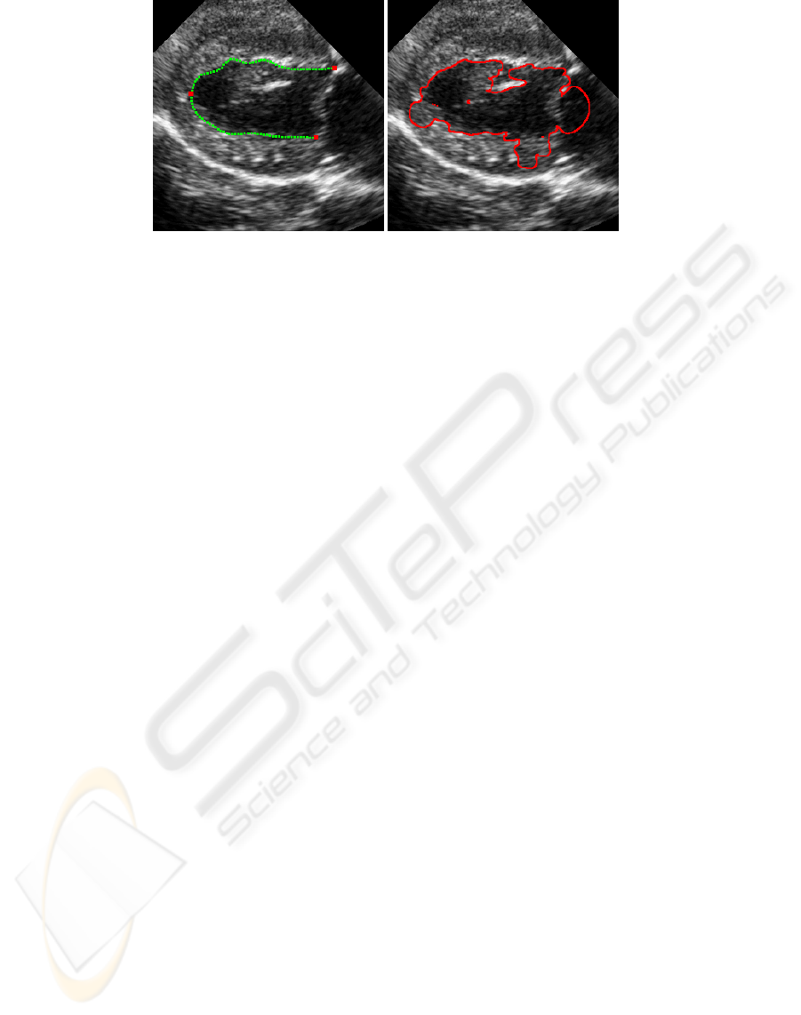
Figure 1: Endocardium detection in an echocardiogram (dog heart). (a) Green: manually drawn ground truth. The red dots

represent the all important valve points and apex. (b) Segmentation using the Geodesic Acrive Contour model. Note the

ruggedness and the leakage through regions of low gradient, while stopping at extraneous anatomical structures inside the

ventricle.

minimized by any of a number of well tested, already

existing minimization algorithms. No special provi-

sions must be made to ensure the numerical stability

of the evolution problem.

2 INTERPOLATION SNAKES

We have argued that parametric snakes are likely to

work better in difﬁcult environments, such as ultra-

sound. Of these snakes, we shall single out one par-

ticular type, most suitable for imposing spatial hard

constraints.

There are situations where certain points or regions

along the boundary of interest have particular signif-

icance for the problem at hand, and so, they have to

be very accurately located. Such is the case, for in-

stance, with the two valve points and the apex of the

left ventricle, in echocardiograms (See Figure 1 (a)).

However, when these spots happen to lie along weak

edges or incomplete data, or simply in a region that

does not differ qualitatively from other regions along

the border, they are nearly impossible to detect by a

“simple-minded” data ﬁtting snake.

Short of implementing special purpose modules

dedicated to the sole detection of these special points,

a compromise solution might be to allow an expert

user to mark these points as ﬁxed at initialization time.

These ﬁxed points are hard constraints for an evolving

active contour and we argue that among the various

types of smooth snakes, interpolation snakes are the

most amenable to imposing hard constraints.

Following (de Boor, 2001), an interpolation spline

is deﬁned in 2D by the following elements:

• a strictly increasing set of real numbers ξ

···<ξ

(the break points),

• a set (with the same number of elements) of data

vectors: y

,...y

∈ R

(the control points).

• a positive integer k (the degree of the spline).

Given this data, the interpolation spline of degree

k, is deﬁned as a curve γ :[ξ

,ξ

] → R

, with the

following properties:

• componentwise, γ is a degree-k polynomial on

each interval [ξ

,ξ

i+1

)

• the pieces ﬁt smoothly at the break points: γ is of

class C

k−1

, i.e. it has k − 1 continuous derivatives.

By ﬁxing the break points and the degree, the

free parameters that deﬁne the spline are the control

points, and these are points on the spline, by deﬁni-

tion. This distinguishes the interpolation splines from

other types of parametric snakes, where the parame-

ters do not have an intuitive geometric signiﬁcance,

and makes interpolation splines suitable for imposing

spatial hard constraints. Indeed, with other types of

parametric snakes, it is not obvious what conditions

should be imposed on what coefﬁcients, in order e.g.

to force the snake to go through a ﬁxed point.

Of particular importance are the cubic interpola-

tion splines (k =3), due to the following property

(de Boor, 2001): among all smooth curves (polyno-

mial or otherwise) that pass through the given control

points at the respective break points, cubic interpo-

lation splines have the smallest total second deriva-

tive, i.e. they are minima of







(τ)



dτ, subject

to the constraints γ(ξ

)=y

for all i. Note that

one minimizes the total second derivative (as opposed

to other derivatives), because of its geometric signif-

icance: under the canonical parametrization, the sec-

ond derivative represents the curvature of γ, and so, it

INTERPOLATION SNAKES FOR BORDER DETECTION IN ULTRASOUND IMAGES

299

measures the amount of bending at each point on the

curve.

The snake energy is a function of the control points:

E = E(y

,...y

), and we ﬁt an interpolation snake

to an image, by varying the control points. Obvi-

ously, if any of these points must remain ﬁxed dur-

ing the minimization, we simply consider the energy

as a function of the remaining control points (but the

spline is still computed through the entire set of con-

trols).

Computation of a cubic interpolation spline is

based on the following lemma. See e.g. “Recipes in

C” (Press et al., 1993):

Lemma 2.1 If γ = γ(t) is a cubic polynomial, then

on any interval [a, b] γ can be expressed uniquely as

γ(t)=A(t) · γ(a)+B(t) · γ(b)

+ C(t) · γ



(a)+D(t) · γ



(b)

(5)

where

A =

b − t

b − a

,B=1− A

C =

− A)(b − a)

,D=

− B)(b − a)

If we take a, b to be consecutive breakpoints, say,

a = ξ

and b = ξ

i+1

, then, since γ(ξ

)=y

and

γ(ξ

i+1

)=y

i+1

are control points (hence given), we

can compute γ(t) for all t ∈ [ξ

,ξ

i+1

], provided we

know the second derivatives γ



at the break points.

The second major point is, therefore, the computa-

tion of γ



(ξ

):=γ



, for j =0,...l− 1. This can be

done by taking the derivative in (5) and requiring that

the ﬁrst derivatives of γ be continuous at the break

points. In the case of a closed spline, this condition

makes sense at all l break points, if we identify natu-

rally y

= y

−1

= y

l−1

and ξ

= ξ

l−1

+ |γ

l−1

We get then a linear l × l system in the unknowns γ



(one system in each dimension of γ) whose matrix has

the form

M =

⎛

⎜

⎝

0 ... 00C

l−1

... 000

0 C

... 000

000... A

l−3

000... C

l−3

l−2

l−1

00... 0 C

l−2

l−1

⎞

⎟

⎠

Lemma 2.2 M has an LU decomposition M = LU .

Proof: The proof is straightforward once we guess

the right form of L and U:

L =

⎛

⎜

⎝

100... 0000

10... 0000

0 b

1 ... 0000

000... b

l−4

100

000... 0 b

l−3

... u

l−4

l−3

l−2

⎞

⎟

⎠

U =

⎛

⎜

⎝

0 ... 00v

0 a

... 00v

00a

... 00v

000 0b

l−4

0 v

l−4

000 0a

l−3

000 0 0 a

l−2

000 0 0 0 a

l−1

⎞

⎟

⎠



In the case of an open spline, the continuity of the

ﬁrst derivative only makes sense at the l − 2 interior

break points, and we set γ



(ξ

)=γ



(ξ

l−1

)=0for

two extra conditions. The resulting system is in this

case genuinely tridiagonal. Thus, in either case, the

second derivatives can be computed in O(l) time. If

the curve is sampled at n points, then computation of

the interpolation spline has complexity O(l + n)=

O(n),asl<n.

3 THE ENERGY FUNCTIONAL

Obviously, since smoothness is built into γ

, we can

drop the internal energy term E

int

from the energy

(3). Our only concerns now are (a) to make the snake

converge to boundaries, (b) keep the points equidis-

tant during the evolution and, eventually, (c) impose

a prior on the overall shape of the snake, e.g. in the

form of a density function on the control vector C,or

using kernel methods as in (Cremers et al., 2003). Un-

der these requirements, we model the snake evolution

by the following energy:

E(C)=



w(s)· < ∇I

⊥



|γ





 

img



||γ



(t)|−1|dt



 

arc

+ E

shape

(6)

Here, <, >denotes the dot product, C =

,...y

l−1

) ∈ R

is again the vector of control

VISAPP 2006 - IMAGE ANALYSIS

300

points of the spline, L = length(γ), and w(s) is a

user-deﬁned weight function along γ.

The image energy E

img

measures the ﬁt to data.

In the simplest case, w ≡ 1, in which case, if we

ﬁx an orientation along γ, the spline will align itself

along edges with dark to its right, and light to its left.

The reason for this is that < ∇I

⊥



|γ



> is minimum,

when ∇I

⊥

is coliniar with γ



and points in the op-

posite direction. This means that the gradient itself

points from right to left as we walk along γ in the

direction of the chosen orientation.

An illustrative example of the general case is shown

in Figure 3. The green curves represent the initial (a)

and ﬁnal (b) interpolation snake. A blue circle rep-

resents a control point with w =0and will be kept

ﬁxed during the minimization. The variable points

are marked in red, either with a plus sign (w =+1)

or with a minus sign (w = −1). The energy (6) is a

function of the red control points only. The weights at

any other point on the spline (green points) are com-

puted by interpolation of the known weights. In this

example, the orientation of the spline is from top to

bottom. Although initialized on an edge, the snake

moves away from it, picking the edges with the po-

larity dictated by the weights: as we walk downward

along the ﬁnal snake (b), the w<0 points are at-

tracted by a dark → light edge, whereas points with

w>0 are attracted by a light → dark edge. This

edge polarity selection by the snake is due to the fact

that unlike the image energy E

img

in (3) which only

depends on the magnitude of the gradient, the E

img

in (6) depends on the magnitude of the gradient and

on the angle between the gradient ∇I and the (unit)

tangent to γ. We have found that this latter image en-

ergy performs better than the original magnitude-only

image energy.

(a) Initial (b) Final

A ﬁnal detail about E

img

is the computation of the

image gradient ∇I. Instead of the usual gaussian

smoothing, or the more sophisticated anisotropic

smoothing methods, we compute the directional

derivatives at each pixel as I

= average(I)

right

−

average(I)

left

and I

= average(I)

bottom

−

average(I)

top

, where each average intensity is cal-

culated on a small rectangle in constant time (only 4

lookup operations, regardless of the size of the rectan-

gle), using a pre-computed integral map of the image

I (Viola and Jones, 2004). Obviously, if a different

amount of smoothing is deemed necessary, the inte-

gral map need not be computed again.

The arclength energy E

arc

is designed to keep the

points of the snake equidistant throughout the mini-

mization process, by penalizing non-arclength para-

meterizations. Since under the canonical parameter s,

the speed along the curve is 1 (i.e. |γ



(s)| =1), then

the amount



|γ



(τ)|−1



is indicative to which extent

τ fails to be the canonical parameter. The necessity of

the arclength term is due to the following argument.

Without exception, a curve γ is discretized by sam-

pling it at equally spaced grid points t

= i·∆t.How-

ever, the points γ

= γ(t

) need not be equidistant, so

this procedure does not correspond to the arclength

parameterization. Of course, if a non-uniform distri-

bution of the points along the snake is allowed, then

the image energy will indicate a misleading measure

of ﬁt, if e.g. a densely populated segment along the

snake happens to fall into an energy pit. It is therefore

crucial to start out with, and maintain equally spaced

points on the snake.

Somewhat surprisingly, the problem of preserving

arclength parametrization along the snake during the

evolution, although noticeable both theoretically and

practically, has been silently overseen. Different ac-

tive contours implementations deal with this problem

in an ad-hoc manner, e.g. by removing points from

regions along the snake where the points have come

too close together, and inserting points in regions

where the snake has become too sparse. The ﬁrst au-

thors to address this problem were, to our knowledge,

Williams and Shah (Williams and Shah, 1992), who

replace the ﬁrst order term in the internal energy E

int

(2), by a term which penalizes for deviations from the

mean distance

d =



|γ

i+1

− γ

|/n along the con-

tour, namely



(|γ

i+1

− γ

|−

d|).

In the discrete setting, we take an equidistant sub-

division of the interval [0,L], namely τ

= i · L/n,

and let γ

= γ

(τ

). We approximate the derivative

at τ

as γ



(τ

) ≈ (γ

i+1

− γ

)/∆τ, and approximate

the arclength energy E

arc

by a Riemann sum:

arc

≈

n−1



i=0



|γ

i+1

− γ

∆τ

− 1



· ∆τ (7)

n−1



i=0



|γ

i+1

− γ

|−∆τ



(8)

If L is chosen to approximate the length of the (ini-

tial) contour, and if this length remains roughly the

INTERPOLATION SNAKES FOR BORDER DETECTION IN ULTRASOUND IMAGES

301

same during the evolution, then

n−1



i=0

|γ

i+1

− γ

|≈L = n · ∆τ

so ∆τ is the mean of all distances between consecu-

tive points along the snake. We arrive this way at the

elastic energy proposed by Williams and Shah.

The initial snake is also constructed so that the sam-

pling at uniform time intervals corresponds to (an ap-

proximate) arclength parameterization. We achieve

this by a judicious choice of the break points ξ

.Ify

are the user-deﬁned control points, then we choose

=0, and ξ

− ξ

i−1

= |y

i−1

| for i>0,so

that the length along the curve between two consec-

utive control points y

i−1

and y

is approximated

∆ξ = ξ

− ξ

i−1

. By choosing the breaks this way,

the usual (uniform) parameter t along the real axis,

becomes - approximately - the arclength parameter

along the resulting spline γ = γ(t). Note that this

choice of the breakpoints, which seamlessly produces

a curve parametrized approximately by arclength, is

not possible with other parametric snakes; it is only

possible with interpolation snakes, because of the par-

ticular signiﬁcance of the snake parameters, as points

on the snake.

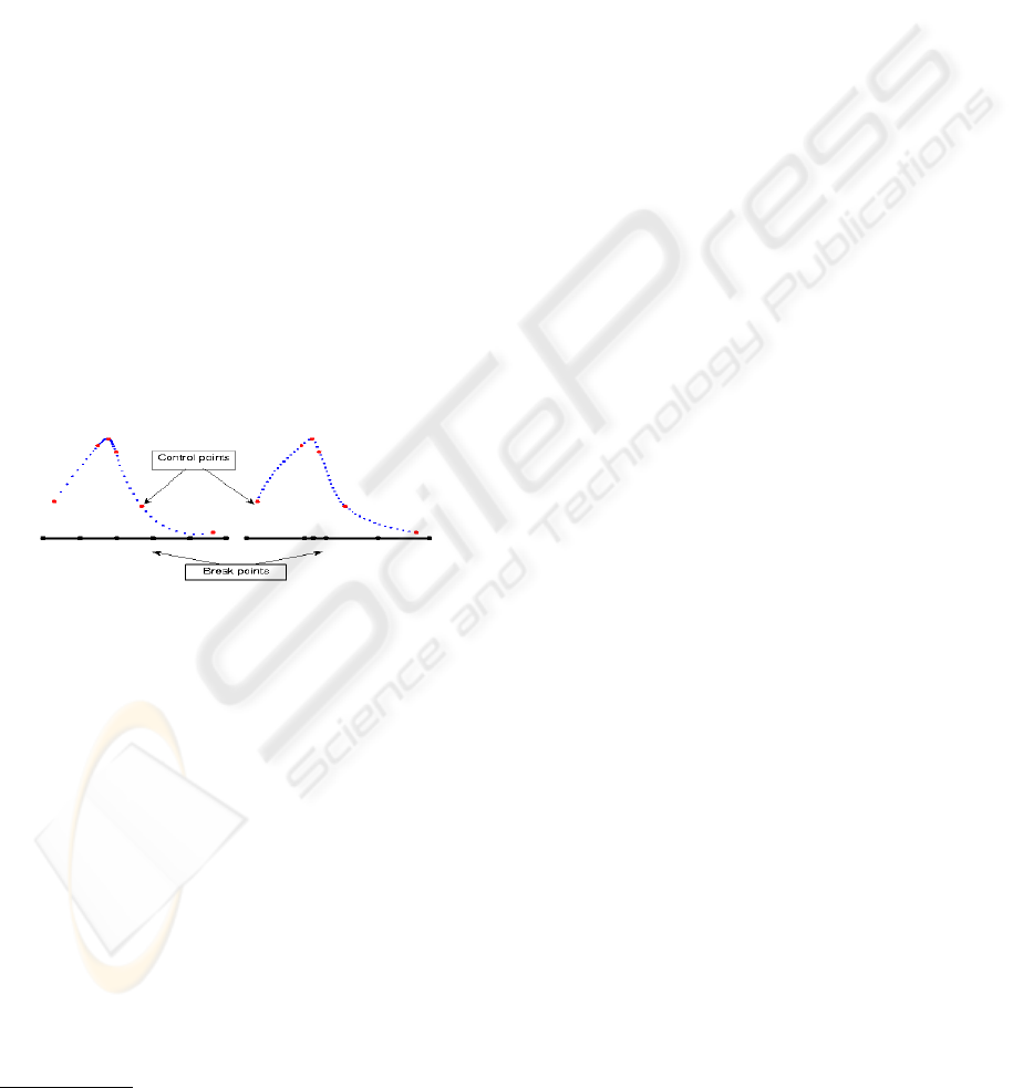
Figure 2: Cubic interpolation spline (blue). Red: control

points. Black: break points. The spline on the left has

equidistant breaks, and is not parametrized by arclength (the

density is higher near points of high curvature). The spline

on the right is built on the same control points as the one on

the left. Choosing the breaks ξ

by ξ

= ξ

i−1

+ |y

i−1

produces an arclength parameterized spline.

The shape energy E

shape

represents the shape

prior knowledge and can be imposed e.g. as a distrib-

ution on the vector of coefﬁcients. Any of a number

of techniques for distribution estimation can be used,

such as e.g. Principal Component Analysis (PCA) on

a number of training contours, Parzen windows, or

more general kernel methods (Cremers et al., 2003;

Cremers et al., 2004). In this paper we use the sim-

plest method: we simply assume a Gaussian distrib-

ution on the control points, estimated using the full

To the extent that the segment y

i−1

approximates the

corresponding arch along the spline.

covariance matrix and the mean of manually anno-

tated training contours. Since the number of control

points is small (e.g. 15 control points), we need not re-

duce the dimension through PCA. We assume known

correspondences on the control points of the training

samples. During the minimization, we factor out the

scale, translation and the rotation of the active con-

tour, by registering it to the mean of the training sam-

ples.

We minimize the energy (6) using Powell’s con-

jugate directions gradient descent algorithm (Press

et al., 1993).

4 RESULTS

A systematic comparison of various active contour al-

gorithms on a signiﬁcant database of (medical) im-

ages is beyond the scope of this paper, and will be

the subject of another study. For now we shall con-

ﬁne ourselves to three examples. We only compare

our interpolation snakes against the geodesic snakes

(Caselles et al., 1997).

Example 1. For this example refer to Figure 3. A

synthetic binary image is used as ground truth (Fig-

ure 3 (a)). We we simulate a noisy boundary by ran-

domly swapping pixels. Figures 3 (b) and (c) show

the initial and the ﬁnal interpolation snake. As be-

fore, the red points are variable, and the blue circles

are ﬁxed points. A single interpolation spline, cannot

make sharp turns, by construction. However, since we

allow for open interpolation snakes, nothing prevents

us from deﬁning a chain of independent snakes (2 in

this example), such that each snake starts precisely

where the previous one ended. Obviously, at the joints

(blue circles) the aggregate snake has no smoothness

(other than continuity), being able this way to simu-

late sharp corners. Figure 3 shows in red the geodesic

active contour. Since it is impossible to keep ﬁxed

points during the evolution of the geodesic snake, the

lower wedge is missed.

Example 2. This example shows the performance

of an interpolation snake vs. a geodesic active contour

in a cardiac ultrasound image. Refer to Figure 4. Parts

(a) and (c) show two signiﬁcantly different initializa-

tions, and (b) and (d) show the detected epicardium.

Part (i) is the geodesic active contour. The rugged

shape and leakage through the boundary are typical

for geodesic snakes (and other non-spline snakes) in

ultrasound.

Example 3. Certainly, our interpolation snake is

not fail proof. It was designed to detect smooth

edges, but, like any other snake, without any fur-

ther constraints it does not have control upon which

edges to detect (other than the polarity of the edges,

as explained in the example in Section 3). For this

VISAPP 2006 - IMAGE ANALYSIS

302

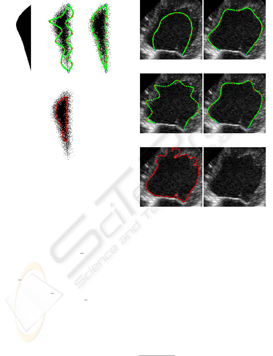
(a) (b) (c)

(d)

Figure 3: Comparison to ground truth in a synthetic image.

(a) Ground truth image. (b) Initialization of a 2-piece ag-

gregate interpolation snake. Each piece starts and ends at a

blue circle (ﬁxed control point). (c) Detected boundary. (d)

Geodesic active contour.

last example refer to Figure 5. Here we incorpo-

rate prior knowledge about the shape of the target

object (ellipse). For training we generate 30 inter-

polation splines z

, 12 control points each, from a

gaussian distribution, whose mean

z approximates an

ellipse. We assume known correspondences between

the control points of any two training samples. If W

is the working snake, then we take E

shape

(W )=

− log N(

z,25)(w) where N(·, ·) is the normal dis-

tribution and w is obtained from W by registering

the latter to the mean

z by a scaling transformation,

using the control points of W and

z. As expected,

using the shape prior, the snake no longer detects ar-

bitrary edges (as in Figure 5 (b)), but only the ellipse

(Figure 5 (d)).

5 CONCLUSION

We have introduced in this paper a new type of active

contour - the interpolation snake - designed to detect

smooth boundaries in very noisy images, with non-

uniform gradient along edges, such as ultrasound.

(a) (b)

(e) (f)

Figure 4: Application to ultrasound. (a) and (c) Initial inter-

polation snake. (b) and (d) Detected boundary. (e) Geodesic

active contour. (f) Original image used in (a)-(e).

This type of snake is in the same category as B-

Snakes. The lack of the compact support property

does not seem to affect the performance of an in-

terpolation snake, while due to the particular signif-

icance of the control points, our snake has other at-

tractive properties, such as arclength parameterization

throughout the ﬁtting process, and the ability to freeze

some of the control points. Prior knowledge can be

introduced naturally, as a distribution on the control

points.

A control point on a B-Snake can change the shape of

the curve only in a local neighborhood, because the basis

functions have compact support. This is not the case with

an interpolation snake.

INTERPOLATION SNAKES FOR BORDER DETECTION IN ULTRASOUND IMAGES

303

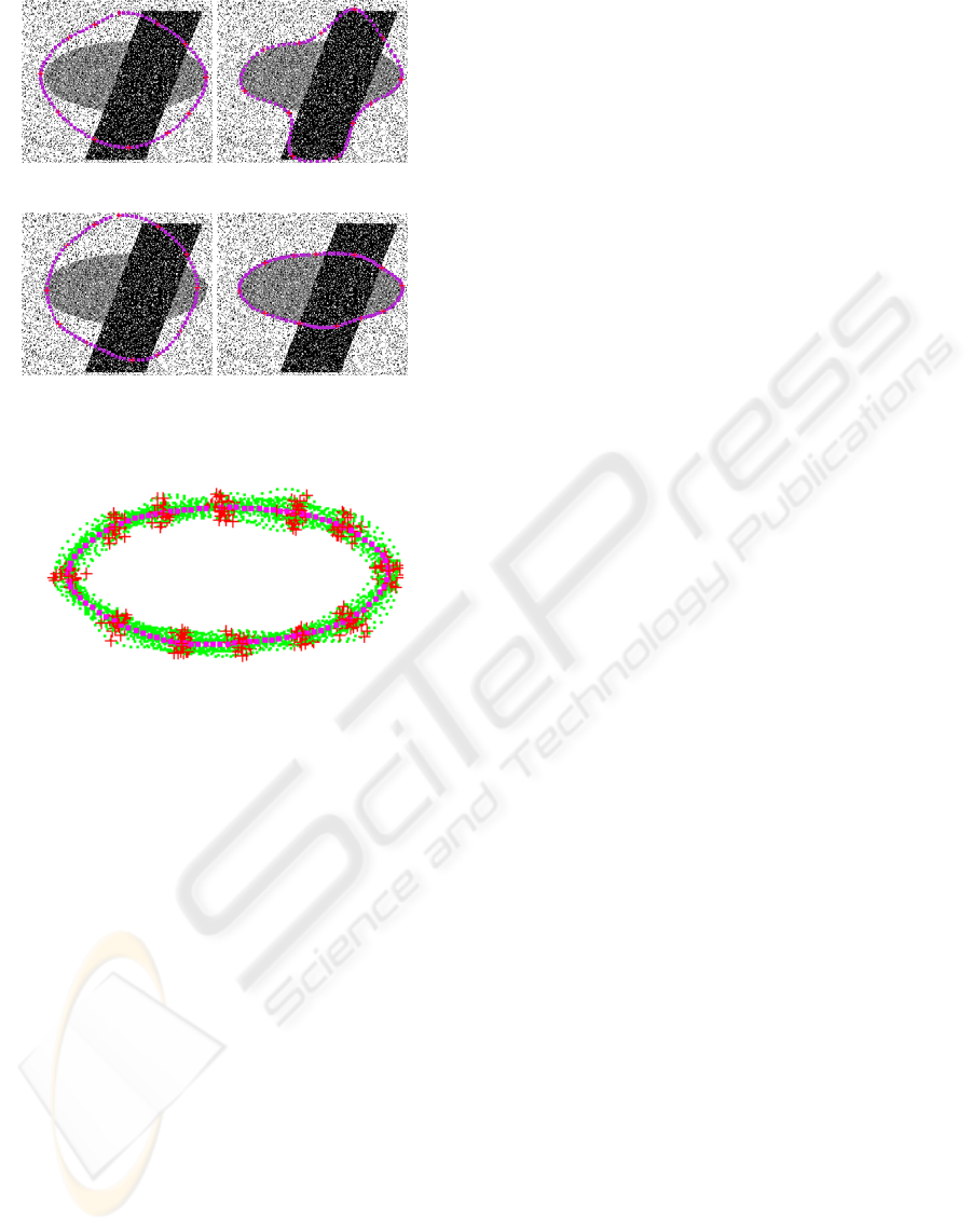
(a) (b)

(e)

Figure 5: Interpolation snakes without shape prior((a),(b))

and with shape prior ((c),(d)). (e) Aligned training contours

(green) and their mean (purple).

ACKNOWLEDGEMENTS

We are greateful to Dr. Bari Olivier and Dr. Au-

gusta Pelosi from the MSU Animal Clinic for pro-

viding us with echocardiograms of the dog heart.

We also thank Kitware Inc. - the producer of the

Insight Toolkit (ITK) - for making publically avail-

able their wonderful software. We have used ITK’s

Geodesic Active Contours.

REFERENCES

Adalsteinsson, D. and Sethian, J. A. (1995). A fast level set

method for advancing interfaces. Journal of Compu-

tational Physics, 118(2):269–277.

Amini, A. A., Weymouth, T. T., and Jain, R. C. (1990).

Using dynamic programming for solving variational

problems in vision. PAMI, 12(9):855–867.

Bascle, B. and Deriche, R. (1992). Feature extraction us-

ing parametric snakes. In Proceedings of the 11-th

IAPR International Conference on Pattern Recogni-

tion, pages 659–663, Netherlands.

Brigger, P., Hoeg, J., and Unser, M. (2000). B-spline

snakes: A ﬂexible tool for parametric contour de-

tection. IEEE Transactions on Image Processing,

9(9):1484–1496.

Caselles, V., Catte, F., Coll, T., and Dibos, F. (1993). A geo-

metric model for active contours. Numerische Mathe-

matik, 66:1–31.

Caselles, V., Kimmel, R., and Sapiro, G. (1997). Geodesic

active contours. International Journal of Computer

Vision, 22(1):61–79.

Cohen, L. (1991). On active contour models and balloons.

CVGIP: Image Understanding, 53(2):211–218.

Cootes, T., Taylor, C. J., Cooper, D. H., and Graham, J.

(1995). Active shape models - their training and ap-

plication. Computer Vision and Image Understanding,

61(1):38–59.

Crandall, M. and Lions, P. (1984). Two approximations of

solutions to Hamilton-Jacobi equations. Mathematics

of Computation, 43(167):1–19.

Cremers, D., Kohlberger, T., and Schnorr, C. (2003). Shape

statistics in kernel space for variational image seg-

mentation. Pattern Recognition, 36(9):1929–1943.

Cremers, D., Osher, S., and Soatto, S. (2004). Kernel den-

sity estimation and intrinsic alignment for knowledge-

driven segmentation: Teaching level sets to walk. Pat-

tern Recognition, 3175:36–44.

de Boor, C. (2001). A Practical Guide to Splines. Springer.

Figueredo, M., Leitao, J., and Jain, A. (2000). Unsuper-

vised contour representation and estimation using b-

splines and a minimum description length criterion.

IEEE Transactions of Image Processing, 9(6):1075–

1087.

Jain, A., Zhong, Y., and Lakshmanan, S. (96). Object

matching using deformable templates. IEEE PAMI.,

18(3):267–278.

Kass, M., Witkin, A. P., and Terzopoulos, D. (1988).

Snakes: Active contour models. IJCV, 1(4):321–331.

Kitware (2005). The Insight Segmentation and Registration

Toolkit (ITK). http://www.itk.org.

Leventon, M. E., Grimson, W. E. L., and Faugeras, O.

(2000). Statistical shape inﬂuence in geodesic active

contours. In IEEE Proceedings of CVPR, volume 1,

pages 316–323, Hilton Head Island, North Carolina.

Malladi, R., Sethian, J., and Vemuri, B. (1995). Shape mod-

eling with front propagation: A level set approach.

PAMI, 17(2):158–175.

McInerney, T. and Terzopoulos, D. (2000). Topology adap-

tive snakes. Medical Image Analysis, 4:73–91.

VISAPP 2006 - IMAGE ANALYSIS

304

Menet, S., Saint-Marc, P., and Medioni, G. (1990). B-

snakes: Implementation and application to stereo. In

DARPA90, pages 720–726.

Osher, S. and Sethian, J. A. (1988). Fronts propagating

with curvature-dependent speed: Algorithms based on

Hamilton-Jacobi formulations. Journal of Computa-

tional Physics, 79:12–49.

Osher, S. and Sethian, J. A. (1990). Recent numerical

algorithms for hypersurfaces moving with curvature-

dependent speed: Hamilton-Jacobi equations and con-

servation laws. Journal of Differential Geometry, 31,

pp. 131–161, 1990, 31:131–161.

Osher, S. and Shu, C.-W. (1991). High-order essentially non

oscillatory schemes for Hamilton-Jacobi equations.

Siam Journal of Numerical Analysis, 28(4):907–922.

Press, W. H., Flannery, B. P., Teukolsky, S. A., and Vet-

terling, W. T. (1993). Numerical Recipes in C:

The Art of Scientiﬁc Computing. Cambridge Univer-

sity Press, 2nd edition edition. available online at

http://www.nr.com.

Rueckert, D. (1997). Segmentation and Tracking in Car-

diovascular MR Images Using Geometrically De-

formable Models and Templates. PhD thesis, De-

partment of Computing, Imperial College of Science,

Technology and Medicine, London.

Sethian, J. (2001). Level Set Methods and Fast March-

ing Methods. Cambridge Monographs on Applied

and Computational Mathematics. Cambridge Univer-

sity Press, 2 edition.

Sethian, J. A. (1996). A fast marching level set method

for monotonically advancing fronts. Proc. Natl. Acad.

Sci. USA, 93:1591–1595.

Staib, L. and Duncan, J. S. (1992). Boundary ﬁnd-

ing with parametrically deformable models. PAMI,

14(11):1061–1075.

Viola, P. and Jones, M. (2004). Robust real-time face detec-

tion. IJCV, 57(2):137–154.

Williams, D. J. and Shah, M. (1992). A fast algorithm for

active contours and curvature estimation. CVGIP: Im-

age Underst., 55(1):14–26.

Xu, C. and Prince, J. (1997). Gradient vector ﬂow: A new

external force for snakes. In CVPR97, pages 66–71.

INTERPOLATION SNAKES FOR BORDER DETECTION IN ULTRASOUND IMAGES

305